None of the solutions to the No Recourse problem that we have investigated are very satisfactory. When uncertainty affects the RHS values of the constraint coefficients, there is always a chance (assuming an unbounded probability distribution) that some constraints will be violated by a fixed solution. Choosing a solution involves a tradeoff between the risk of infeasibility and the expected value of the objective function. The simple recourse model proposes costs of exceeding or falling below the resource amount and finds the optimum solution considering the original objective function and the expected penalty cost. This eliminates the necessity of specifying risk levels, but adds the requirement of accessing penalty costs.

Deterministic Equivalent

To explain the simple recourse approach, we consider the linear programming model below. We show a tilde over the RHS vector to indicate that its components are random variables with known probability distributions. We use a minimization objective function for the convenience of the discussion. The methods work equally well for ">=", "<=" and "=" constraints.

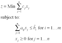
The problem, as stated, is not well defined because it does not indicate the time order of decisions and random variable realizations. Also, it does not specify the response of the decision maker when the resources requested by a solution exceed or fall below the amounts available. These issues are addressed on this page.

The decision maker must choose the values of the variables, x, before the random RHS values are known, so this is similar to the no-recourse situation discussed on the previous pages. This situation is, however, a special case of the decision making with recourse problem to be considered later, so we use the term simple recourse to describe this case.

The model below introduces new variables expressed by the vector z, where is the amount of resource i used by the solution. The constraints assure the equality between the amount of resource used, and . After the decisions have been made and after the random RHS values are realized it may be that the amount of resource used for some constraint i, , may be different than the amount available, . In that case we will assess a penalty based on the difference between of the amount used over the amount available. We cannot be sure of the value of the penalty when the decisions are made, but we can compute the expected value. A reasonable goal for the decision maker is to minimize the expected value associated with the decision. This is reflected in the model.

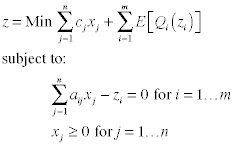
The new term in the objective is the expected cost of the resource used. We call it the expected recourse cost. We will derive a closed form expression for the expected recourse cost, so that the model can be solved as a deterministic equivalent math programming model. When the probability distributions for the RHS values are discrete, the representation of the expected value is piecewise linear, and it can be solved as a linear program. When the distributions are continuous, the model is a separable nonlinear math programming model. The expected recourse cost is a convex function of .

On this page we concentrate on the discrete distribution case. On the next page we show how to approximate a continuous distribution with a discrete distribution. In the following we assume that the random variables are independent, but the results can be extended to dependent random variables.

Expected Resource Cost

For a particular realization of the random RHS and a particular selection of , the resource available is either exceeded by the requirements or falls below the requirements. We propose a linear penalty for both events. In the following we write the expression for the expected recourse cost.

Any kind of linear constraint can be modeled with appropriate costs of shortage and overage. For a "<=" constraint the shortage cost would be positive and the overage cost would be zero. For a ">=" constraint the shortage cost would be zero and the overage cost would be positive. For an "=" constraint both shortage and overage cost would be positive. For many practical situations, both costs are nonzero, but a requirement of the analysis is that the sum of the unit shortage and overage costs be positive.

To find an expression for the expected recourse cost we must consider the distribution of the random RHS values. Here we assume a discrete distribution. In the following we drop the constraint subscript, but it will return later. The distribution is defined by a set of K values of the random variable each with a possibly non-zero probability. Values not enumerated have zero probability.

For discrete distributions the expected values can be determined by summing.

Combining these relations we find a useful result that allows the determination of one of the expected values given the other.

To construct the model we must divide the amount of resource used into pieces.

It can be shown (but not here) that the expected shortage and overage costs, and hence the expected recourse cost can be computed by a piecewise linear expression.

Combining these relations we obtain an expression for the expected recourse cost.

Math Programming Model

Finally we replace the expected recourse cost with the piecewise equivalent in the math programming model. Subscripts have been added to represent the expected costs for the several constraints.

When the uncertain RHS values have discrete probability distributions, the equivalent math programming model is linear, and the model is relatively easy to solve. The number of variables is increased by the number of pieces used to represent the expected recourse costs. The constraints are increased by those relating the resource usage to the sum of the pieces and simple upper bounds on the pieces of the expected value representation. The latter don't add materially to the computational difficulty.

Small Example

To illustrate the method we use a product mix problem with only four products and two resources. The details of the problem are described on another page. The problem has four products with production amounts as x1 through x4. The unit profits for the products are in the objective coefficient row. The problem has two resources, carpentry and finishing. The hours used for the products on the resources are shown in the constraint matrix. The available hours for the resources are uncertain. The numbers shown as the RHS values are the expected values. The solution shown solves the expected value problem.

To address the stochastic problem we must know the probability distributions for the resource availabilities. The possible values of the hours available are shown in the table. The values are equally likely, so each has a 0.25 probability.

When the number of hours available for the resources happens to be less than the amount used by the production plan, there is a shortage of hours and extra hours must be purchased to make up the shortage. The cost of extra carpentry hours is $5 per hour and the cost of extra hours for finishing is $10 per hour. There is no penalty for when the available hours exceeds the amount used (overage).

The Math programming model for the simple recourse problem is below. Two constraints represent the resource requirements and two provide the piecewise linear expected recourse cost. The rows of the worksheet starting at row 20 compute the upper bounds and objective coefficients for the pieces of the expected recourse cost. The optimum solution produces more than the expected value solution and there is some chance that extra carpentry hours will be purchased. The solution uses fewer finishing hours than the smallest value of the finishing resource, so there is no chance that extra finishing hours will be purchased.

Side Model