 |

|
The add-in computes approximate values for
the steady-state measures when the arrival or service processes
are not required to have exponential distributions.
To add a non-Markovian Queuing model
on the worksheet, place the cursor at a cell where the model
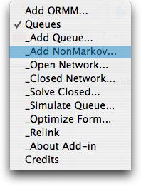
is to be described and select Add NonMarkov from the
menu. The dialog box below allows entry of the parameters of
the model. This model does not require the interarrival and
service distributions to have exponential distributions. Rather,
the model requires the specification of the coefficients of
variation (COV) of the arrival and service processes. The COV
for arrivals is the standard deviation for time between arrivals
divided by the mean time between arrivals . For an exponential
distribution the COV is 1. Distributions with less variability
than the exponential have COV < 1, while distributions with
more variability have COV > 1. The service process COV is
the standard deviation of the service time divided by the mean
service time. |
Example: An order picking process |
| |
An order picking process in a warehouse gets calls
for service at an average rate of 8.5 per hour. The average
time to fill the order is 0.1 hours. For analysis purposes
assume both times are exponentially distributed. Analyzing
the system as an M/M/1 queue, the average time in the
queue is 0.5667 hours. An opportunity arises to reduce
the variability of the process for filling orders. The
inventory manager wonders if the change is worth the
cost.
To analyze this problem we select
the NonMarkov option from the menu. The dialog below
defines the parameters of the model. The name, arrival
rate, service rate and number of channels are entered
in the appropriate boxes. The approximation does
not apply to finite queues or finite populations,
so these options are not present. If the replication
entry is greater than 1, the number entered determines
the number of Queuing models put on the worksheet.
We illustrate the presentation of three replications
below. |
|
| |
|
| |
The
check boxes on the dialog determine optional presentation
of the steady state results. Checking the Show Titles box
causes titles to be added to the worksheet. When defining
a series of Queuing models in sequential cells, it is useful
to show the titles for the first model, and then skip the
titles for the remaining models.
The set of results for the Non-Markovian
case is smaller than those available for Poisson queues.
This is partially due to the restriction against finite queues
and finite populations, making some results not relevant.
The approximations used do not allow the computation of state
probabilities.
The results for three replications of the Queuing model are
shown below. When the models were created on the worksheet
all had the default parameters shown for PP1_1. To illustrate
the effect of reducing the variability in the service times,
we set the COV to 0.5 in the second model and 0 in the third
(no variability). In general the numbers and time in the queue
decrease as variability decreases. Note that with COV of 1,
the distribution is actually Markovian (Poisson process). Thus
we see an M in the type designation when the COV is 1.
It is clear from the results that reducing variability in
the service process causes decreased time in the queue. The
mean time in service does not change because that is fixed
by the data and unaffected by the variability. |
| |
|
Using Reduced Variability to Obtain more Throughput |
| |
| We wonder whether the benefits of the reduced variability
could be used to obtain more throughput, rather than reduced
queues. That is, we want to increase the arrival rate in
the second two systems to obtain a time in the queue equal
to 0.567. This is indeed possible as shown in the analysis
below. Note that for the systems in columns I and J, the
arrival rates have been increased substantially while the
time in the queue remains at 0.567. |
|
| |
|
| |
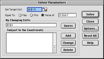
This
analysis was performed using the Excel Solver, called with the
Solver command on the Tools menu of Excel. The Solver dialog
shown below is set up to obtain the solution in column I above.
The target cell, I13, holds the mean time in the queue.
The changing cell, the cell I3, holds the arrival rate.
We have asked Solver to find the value of the arrival rate that
gives a mean queue time of 0.5667. When performing the analysis
it was necessary to give an initial value larger than the ultimate
solution of 9.006. With a smaller initial value, Solver tried
arrival rates greater than 10 and the procedure stopped because
the system is unstable for arrival rates greater than 10.

|
Reducing
Variability of Both Arrival and Service Processes |
| |
Reducing
the variability of both the interarrival times and service times
further reduces the time in the queue as shown below. The results
of column N show that by cutting the COV to 0.5 reduces the queue
time to 1/4 of its value with Poisson processes. Reducing the
COV's for both processes to 1/10 the original value reduces the
queue time to 1/100 of its former value. |
| |
|
| |
Again
we investigate the possibility of increased throughput while
keeping queue time as a constant. We used Solver as previously
described to obtain the results below. The arrival rate for the
third case is at almost the theoretical maximum of 10. |
| |
|
| |
When
both COV are equal to 1 the system can be analyzed with no approximation
using the Poisson queuing formulas. The formulas used by the
Non-Markovian analysis are also accurate for M/G/1 systems. For
all other systems, the results are approximate. |
| |
|


