|
|
 |
Simulation |
 |
-
Inventory Model |
 |
 |
Here we illustrate the second model type available, the inventory
model. The simulation describes a reorder point - lot size
system. The inventory holds a single product and is reviewed
periodically, weekly for the example. The inventory level is
decreased by demand described as a random variable. When
the inventory level reaches some reorder point specified as
a parameter, an order is placed. The amount of the order is
also a parameter of the simulation. After a predetermined lead
time, the replenishment is delivered and added to the inventory.
During the lead-time, the inventory may be exhausted and shortages
may occur. We assume that shortages are backordered and satisfied
when the next order is delivered. An option models the lost
sales case.
There are costs associated with replenishment, backorders
and inventory level. We will construct a simulation of this
situation. The goal of the analysis might be to choose a reorder
point and lot size that minimizes the average daily cost. Simulation
does not answer that question directly, but it can be used
to evaluate alternative choices.
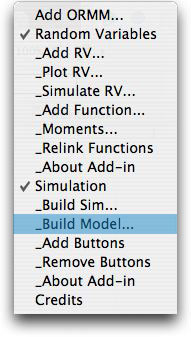
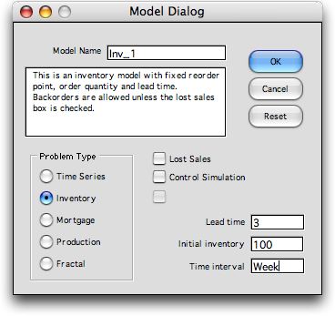
The model is constructed by choosing the Build Model command
and filling in the dialog that is presented. The model name
can contain no spaces or punctuation. The name is used to
identify various ranges on the worksheet and cannot be changed
after the worksheet is constructed. The default is to backorder
shortages, but the lost sales model is obtained if
that box is checked. The Control
Simulation box
operates the inventory one period at a time and the user makes
reorder decisions. The initial inventory is entered as a parameter,
but it may changed on the worksheet. The lead-time affects
the simulation structure and once it is defined here it cannot
be easily changed.

|
The Worksheet Model |
| |
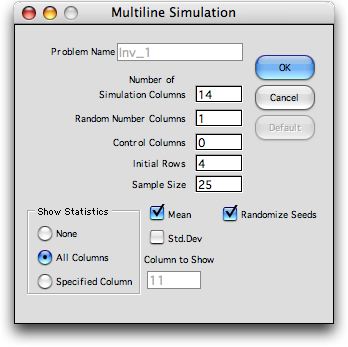
Pressing the OK button
on the model dialog, brings forth a second dialog that provides
the features of the multiline simulation model that will describe
the process. The problem name is fixed as the name given in
the Model dialog and the parameters are set to their proper
values. The numbers of columns may be increased to accommodate
additional model features, but they should not be reduced or
the program will not be able to build the inventory model.

As the worksheet is constructed, a third dialog
will ask for the distribution of the demand. For the example
we suppose that the demand is normally distributed random variable
with mean 25 per week and a standard deviation of 5. Pressing
OK for this dialog, builds the worksheet for the inventory model.
All expressions are automatically placed in row 1 and the random
variable and parameter definitions are placed on the worksheet.
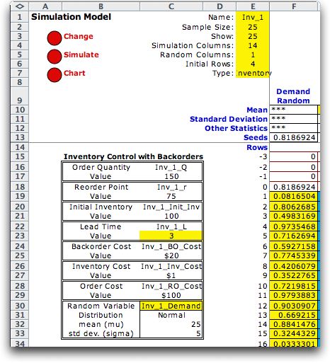
The figure at the left shows the top corner of the worksheet.
The buttons control the operation of the simulation. |
| |
 |
The parameters of the system are placed in columns B and
C starting at row 16. The order quantity (C17) and reorder
point (C19) are the decision variables. The initial inventory
is in C21 and the cost parameters are in C25, C27 and C29.
The mean and standard deviation of the demand are in C32
and C33. All these numbers may be changed to represent
the system under study.
The
lead-time parameter in C23 is shown in yellow. This indicates
that the lead-time should not be changed. Changing
the lead-time in C23will not affect the results because
it is fixed in the expressions defining the system. If you
want to analyze the system with a different lead-time,
create another model.
The seed in F13 is used for Monte Carlo simulation. It
controls the sequence of demands realized for the simulation.
Clicking the Simulate button changes the seed
and produces a new simulation run.
The Change button controls aspects of the simulation.
An option useful here is the number of observations in
the simulation. The Chart button produces a chart
of one of the simulated columns.
|
|
| |
At the top of the worksheet
are simulation parameters in columns E and I. Results for the
simulation run are in column L. |
|
| |
The simulation model
is shown in two parts below. This model has a single random variable
for demand governed by the simulated values in column F. The
columns necessary for the simulation are columns G through T.
The model is simulated for 25 weeks, but only the first five
weeks are shown. The interesting result is in column T that shows
the cost per week. The other columns are necessary to determine
the replenishment orders, backorder amounts and inventory amounts. |
|
| |
The initial conditions
are in the rows labeled -3 through 0. The only nonzero value
shown is in cell K10. This cell holds a formula that links its
value to the initial inventory level in cell C21. |
|
| |
The cells in column V,
W and X summarize the results for the 25 simulated weeks. |
|
Row 1 |
| |
The simulation is implemented
by the formulas in table row 1, Row 19 on the worksheet. To create
the other rows of the simulation, we simply perform the Excel
function Fill Down on the simulation form. In this way
all the rows have the same formulas as row 1, but displaced in
reference. A few of the cells are named for the formulas.
- Inv_1_Demand is the range {C31...C33}. This range identifies
the normal distribution for the demand and specifies the
mean and standard deviation.
- Inv_1_r is the number in cell C19. This is the order point.
When the inventory position reaches the order point an order
must be placed.
- Inv_1_Q is the number in cell C17. It is the order quantity
that is placed at each replenishment order.
- Inv_1_BO_Cost , Inv_1_Inv_Cost, and Inv_1_RO_Cost are in
C25, C27 and C29 respectively. They are the cost parameters
for the inventory system.
|
Column |
Quantity |
Formula |
F |
Demand Random |
=SIM_rand(-F18) |
G |
Beginning Inventory |
=K18 |
H |
Delivery |
=O15 |
I |
Inventory + Delivery |
=G19+H19 |
J |
Demand |
=MAX(ROUND(RV_sim(Inv_1_Demand,-F19),0),0) |
K |
Ending Inventory |
=I19-J19 |
L |
On Order |
=L18-H19+O18 |
M |
Inventory Position |
=L19+K19 |
N |
Reorder |
=IF(M19<=Inv_1_r,1,0) |
O |
Order Quantity |
=IF(N19=1,Inv_1_Q,0) |
P |
Inv. Less Shortages |
=I19-J19 |
Q |
Fraction Backorder |
=IF(I19>0,IF(P19>0,0,-P19/ABS(J19)),IF(P19>0,-I19/ABS(J19),1)) |
R |
Back Orders |
=IF(Q19=1, -K19 -P19 /2,-MIN(K19,I19 )*Q19/2) |
S |
On Hand |
=IF(Q19=0, K19 +J19 /2,MAX(K19,I19 )*(1-Q19)/2) |
T |
Cost |
=S19*Inv_1_Inv_Cost + R19*Inv_1_BO_Cost + N19*Inv_1_RO_Cost |
|
|
| |
We identify several
interesting cells in row 0 and row 1.
Cell |
Description |
I18 |
This cell holds the initial inventory
amount. It may be changed, as well as the other cells in
the initial rows of the model. |
H19 |
This cell is interesting because
it points several rows higher (earlier) in the simulation.
Cell H19 represents the replenishment amount received in
day 1 and points to the order quantity that occurred four
days earlier (in cell M15). We are assuming here that orders
are placed at the end of the day and are available for
sale three whole days later. The amount will be available
for sale during the fourth day following the order.
In general, expressions may point to any cell that describes
the system earlier in time. It is necessary to provide
one more initial row than the lead-time. Otherwise the
expression would point to a non-numerical cell.
Expressions may also point to cells in row 1. It is good
practice to only point to cells to the left in row 1. Otherwise
it is possible to create circular references. Excel does
not allow this. It is not reasonable to point to cells
lower (later) in the simulation. Circular references will
almost certainly be created. |
N19 |
This cell holds an "IF" expression,
that returns 1 if the inventory position in cell M19 is
less than the reorder point. Thus it indicates if an order
will be placed. |
O19 |
This cell holds an expression
that places the order quantity into the cell if the previous
cell, N19, is 1. |
T19 |
This cell computes the cost
per day based on the cost parameters and the decision to
order, the backorder amount and the inventory amount. Both
of the latter are computed at the end of the day. |
|
| |
By increasing the
sample size, the model can be simulated for a large number
of days to determine the average cost of operating the inventory.
The figure below shows the results of 1000 observations with
a reorder point of 75 and an order quantity of 150. A number
of rows and columns are hidden for clarity. Whenever the ending
inventory plus the amount on order is less than 75 and order
is placed. The order amount is 150.
At the top of the worksheet, the add-in has added summary
information about the simulation run. The cost of this policy is
$111 per week. To use the simulation for decision making, we
would vary the reorder point and order quantity to minimize
the total cost. Since the simulation is dynamic, this can be
done without rebuilding the model. |
|
| |
This model has been implemented
as the Inventory Game using the Control option.
The student observes the results at the end of each week and
makes real-time decisions regarding the inventory policy. |
| |
|
|


