Predefined models are reached by choosing Build Model from the Simulation menu.

The model dialog appears with a list of model types currently available. Four model types are currently available. In this section we describe the Time Series model. Checkboxes determine if the series should have a trend component or a step component. We illustrate below the case when both are chosen.

The mathematical model describing the situation is shown below. Note that the trend component is accumulated since the beginning of the simulation with the sum term. The step component is a quantity added to the base demand at each iteration.

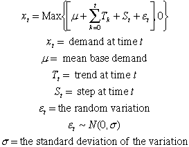
The trend component is itself a random variable described in the following.

At each iteration, the trend is the trend value at the previous iteration plus a new trend added in the current iteration. The addition is from a Normal distribution with a specified standard deviation and a mean of 0. However, whether the current value is added or not depends on a Bernoulli random variable taking on the value 0 or 1. The Bernoulli distribution has the probability parameter given as 0.1 specified on the dialog.

In practice, this represents a situation where the series is affected by random influences that either causes a trend change or not. The probability of the change is given by the parameter of the Bernoulli distribution.

The step component is similarly affected by a random variable with a Bernoulli distribution. It represents some shock that affects the constant term added to the base demand. The model for the step component is similar to the trend component, but it is affected by different random variables.

Although this model seems complicated, it might represent a situation where demand is not constant over time. Such a model could be a useful start for a variety of situations involving time series.

The Worksheet Model

Pressing the OK button on the model dialog, brings forth a second dialog that provides the features of the multiline simulation model for the process. The problem name is fixed as the name given in the Model dialog and the parameters are set to their proper values. The numbers of columns may be increased to accommodate additional model features, but they should not be reduced or it will not be possible to build the time series model. The sample size is selected here to illustrate the affects of trend and step changes.

Pressing OK for this dialog, builds the worksheet for the time series model. All expressions are automatically placed in row 1 and the random variable definitions are placed on the worksheet. Dialogs are presented for each random variable, so the user can select the types and parameters of the distributions. The figure below shows the random variable definitions, which are placed in columns B and C. The parameters of the distributions can be changed to suit the situation.

Row 1 for the Simulation