The production model is adapted from a story in The Goal by Goldratt. We first describe the story and then use the add-in to model the more general sequential production process. The story involves three boy scouts playing with matches. The game involves throwing dice and passing matches from one boy to the next. The scoutmaster is at the end of the line trying to light a fire with the matches produced by the third boy.

We start with a big pile of matches to the left of the first boy. Boy 1 throws a single die. The number showing is his production, so in this case the first boy produces 4 matches. These matches are the raw materials for the second boy.

The second boy throws the die. His production capability is the amount shown on the die, but he can only produce as much as available from the first boy. His production is the minimum of his capability or the number remaining from the first boy. There are 4 matches available, but the capacity of the second boy is only 2. He passes these to the third boy, leaving 2 matches remaining. These two are called work in progress (WIP).

The raw materials for the third boy are the matches provided by the second boy. Again, he produces the minimum on his die or the matches available. For this case the capacity of the third boy is 5, but only 2 matches are available as raw material. The remaining 3 units of capacity are wasted. This is disappointing to the third boy because his capacity was so much greater than his production. There is no additional WIP.

The scoutmaster has a demand that also depends on the throw of the die. For the first iteration, the scoutmaster demands 4 matches. The third boy has only produced 2, so the scoutmaster takes these two. The unsatisfied demand is lost. The scoutmaster is disappointed with the third boy who seems to be the bottleneck in this system.

In this first iteration, the system produces 2 matches. Two matches remain in the system as WIP waiting for processing by boy 2. This WIP has already been processed by boy 1 and is available to boy 2 for processing in the next iteration.

Goldratt told this story to illustrate the negative effects of statistical variation on a serial production line. The simulation model allows the system to have as many stations as desired and the statistical variation to be governed by any of the common probability distributions.

The Excel Model

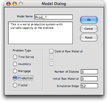
This story describes a serial production system with a specified number of stations. To create the model in Excel, click the Production button on the model dialog. The dialog has a field for Number of Stations. The checkbox adds a feature to the model that controls the flow of raw material into the system. This is illustrated later. The Raw Material Supply field is only relevant if this box is checked.

After clicking OK, the multiline dialog will be presented. Click OK. Then a series of dialogs will be presented asking about the probability distributions of the production amount at each stage. The uniform distribution representing the throw of a single die is the default. The add-in finally constructs a spreadsheet model of the multistage process. We illustrate the features below.

Parameters

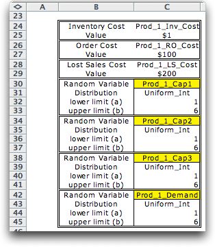
The cost parameters of the model are below. We assume that an iteration reflects a one-week interval. The first three entries are the cost parameters. The inventory cost is the per unit cost of WIP per week. The cost does not depend on the location of the WIP in the process. The order cost is the cost of placing a nonzero order for raw materials. For the example, this cost is expended in every week. It is relevant when manual control of reorders is controlled manually. The lost sales cost is the unit cost of demand that is unmet by production.

We have chosen the integer-uniform distribution for demand and production capacities. The integer-uniform distribution models the throw of a die.

Worksheet

The worksheet illustrates a three-station example. Station 1 accepts raw material, performs its operation and then passes the material to station 2. Station 2 performs a second operation and then passes the material to station 3. After the operation at station 3 the material enters a finished good inventory. The demanded quantity is withdrawn from this inventory. If demand is greater than the amount available, lost sales are experienced. Because it has so many columns we present the worksheet in two parts.

Columns G through J hold the random numbers that govern the capacities for the three stations and the finished good demand. Column K holds the materials purchased in each week. For the example, the purchase amount is exactly the capacity of the first station. The input capacity is unlimited.

The station 1 information is outlined in blue. We review the equations for period 1, row 17 on the worksheet. Column L holds the input WIP. It is equal to the output WIP of the previous period. Cell L17 holds a formula that is "=P16". Since station 1 always produces its capacity, the WIP is always 0. Column M holds the amount of material available for production "=K17+L17". Column N holds the capacity for production. This is a random amount taken from the RN1 random variable "=RV_sim(Prod_1_Cap1,-G17)". Column O holds the actual production, "=MIN(M17,N17)". Column P holds the WIP available for the next period, "=M17-O17". The results of station 1 are not too interesting, given that it produces an amount equal to its capacity. Station 2 has more interesting results. The formulas for station 2 are the same as for station 1, but the columns references are advanced by 5.

The columns for station 3 and the finished goods inventory are below. The formulas again are similar to stations 1 and 2. Columns AF compute lost sales, "=MAX(0,AC17-AD17)", total WIP, "=L17+Q17+V17+AA17", and total cost, "=AG17*Prod_1_Inv_Cost+IF(K17>0,Prod_1_RO_Cost,0)+AF17*Prod_1_LS_Cost".

To the right of the station and demand simulation we see summary results for the 52 weeks simulated. Although the mean production capacity at each station is 3.5 per week, the average sales per week is just above 3. The average demand is 3.5 per week, so the lost sales are about 0.5. The average WIP per week is about 20.4. The average time required for a match to move from station 1 to sales is the cycle time. By Little's Law:

Cycle Time = WIP/Sales

For the example the average cycle time is about 6.8 weeks.

The results indicate that the sequential production process with statistical variability is not very efficient. The effect of reducing variability is illustrated when we change the lower and upper limits on the uniform distributions to 3 and 4. The random variables have the same mean values but much less variance. The system results shown below are much better.

With integer variables we cannot reduce the variability to zero and maintain a mean value of 3.5 per week, but we can set the lower and upper limits to 4. This eliminates variability, and results in an average production rate of 4. When variability is eliminated, lost sales, WIP and cycle time all go to zero.

In this model, the minimum cycle time is 0, because material does not enter inventory if it passes through the system in a single period.

Controlling Raw Material Flow

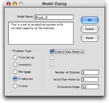
One suggestion for controlling a system such as this is to control the input flow of raw material. This is an option available for the model. To investigate this option click the Control Raw Material box.

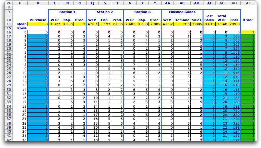
With the control option a new column is included in the model shown as column AI below. The column shown in green is the order quantity that will be delivered in the next period. When the worksheet is created this column has zero's except for the yellow entry at the top. We have filled in the column with the value 3. This puts a steady flow of 3 units into the system at each period.

The results of the 52-week simulation are below. Since the average demand is 3.5, there will be lost sales. Because of statistical variability there is still a considerable amount of WIP and cycle time is greater than the minimum value of 0.

• What is the effect of reducing the variability of the production capacities?
• What is the effect of having more production stations? The model allows the analysis of any number of stages.
• If one were to add more capacity, would be better at the beginning of the line or at the end? Capacity is added by increasing the upper range on the uniform distribution.
• Can a similar simulation be constructed for a pull system of production, rather than the push system illustrated here?
• Using the control column, how would you model a CONWIP inventory policy? This policy orders raw materials in exactly the amounts sold in each period. The WIP remains constant at the initial value throughout the simulation.
• Would it be useful to adopt an order level-order quantity policy? In some periods the order quantity could be zero, thus reducing the reorder cost.

The Game