|
|
>  |
Teach
Dynamic Programming Add-in
|
 |
-
Problem Models
|
|
 |
The add-in comes with a series
of problem-specific models as well as a general
model that allows
the construction of DP models constructed by
the student. In this and the following pages
we describe each of the built-in models. This
page describes the model for the knapsack problem
in some detail. Other models are described in
general terms but with less detail on the DP
implementation.
The examples for this section are in the Teach
DP demo (teachdpdem.xls). The specific models
are described in the PDF supplement, Dynamic
Programming Models (dp_models.pdf). To solve
or change the model you must have the Teach
DP add-in loaded. Use the Relink buttons command
to establish links to the worksheet buttons.
|
|
Example Problem |
| |
To illustrate using a built-in model
we use the Investment Problem considering in the Models
section of the site.
A portfolio manager with a fixed budget of $100 million is
considering the eight investment opportunities shown in the
table below. The manager must choose an investment level for
each alternative ranging from $0 to $40 million. Although an
acceptable investment may assume any value within the range,
we discretize the permissible allocations to intervals of $10
million to facilitate the modeling. This restriction is important
to what follows. For convenience we define a unit of investment
to be $10 million. In these terms, the budget is 10 and the
amounts to invest are the integers in the range from 0 to 4.
Table 1 provides the net annual returns from the investment
opportunities expressed in millions of dollars. For example,
an investment of $10 million in opportunity 1 provides an annual
return of 4.1 million. When time value of money is considered
this 4.1 would be considered the uniform annual equivalent
of the opportunity.
A ninth opportunity, not shown in the table, is available
for funds left over from the first eight investments. The return
is 5% per year for the amount invested, or equivalently, $0.5
million for each $10 million invested. The manager's goal is
to maximize the total annual return without exceeding the budget.
Table
1. Returns from Investment Opportunities |
Amount |
Opportunity |
Invested
($10 million) |
1 |
2 |
3 |
4 |
5 |
6 |
7 |
8 |
0 |
0 |
0 |
0 |
0 |
0 |
0 |
0 |
0 |
1 |
4.1 |
1.8 |
1.5 |
2.2 |
1.3 |
4.2 |
2.2 |
1.0 |
2 |
5.8 |
3.0 |
2.5 |
3.8 |
2.4 |
5.9 |
3.5 |
1.7 |
3 |
6.5 |
3.9 |
3.3 |
4.8 |
3.2 |
6.6 |
4.2 |
2.3 |
4 |
6.8 |
4.5 |
3.8 |
5.5 |
3.9 |
6.8 |
4.6 |
2.8 |
|
Problem Definition |
| |
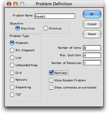 |
Selecting the Model option from the Teach_DP menu
presents the problem definition dialog.
Fields accept the problem name and relevant
parameters. Clicking a button on the left
selects one of the problem types built into
the program. We recognize the investment
problem as a knapsack problem with the opportunities
equivalent to items. The resource is the
budget limitation. We click the Nonlinear box
because the investment returns are not linear
with the amount invested.
The names of the fields at the right side
of the dialog a affected by the problem type
selected. The first checkbox label (here
labeled
Nonlinear) also depends on the type.
When checked, the Make Random Problem box
fills in the data form with random numbers
appropriate to the problem type. Of course,
these may be changed on the worksheet. The Show
Comments adds a small red label to some
of the cells of the worksheet.
|
After entering data and pressing the OK button, a worksheet
is created with the name specified in the dialog. Many ranges
on the worksheet are given Excel names with the preface being
the worksheet name, so that name should not be changed after
the worksheet has been constructed.
In the greater part of the worksheet the program constructs
the dynamic programming model consisting of the state and decision
definitions and all of the other components required for dynamic
program. The
problem specific data is placed to the right. We have entered
the data for the example in the tables provided.

|
| |
At the top of the
worksheet we see a variety of information describing the problem,
solution process, interaction and display. The Solve button
initiates the dynamic programming solution process.

|
| |
Without any knowledge of the DP
model, the user can click the Solve button to obtain
the solution below. Statistics of the solution process start
in column M. |
|
| |
Since the Graph option has
been chosen, the solution presents a graph of the state space.
There is a single initial state at (1,0). The nodes colored blue
are the final states. The gold colored states and the heavy lines
indicate the optimum path through the state space. The red lines
indicate the optimum decisions for the states. The total number
of states with exhuastive enumeration has 88 states with S1 between
2 and 9 and S2 between 0 and 10. The single initial state provides
the total number of 89. |
| |
|
Excel Model |
| |
A DP model uses states and decisions
to describe a sequential decision process. A number of functional
expressions define the beginning, middle and end of the process.
A quantitative measure determines the costs and/or benefits
of the process.
When using this DP add-in for Excel, the expressions describing
the model must be placed into cells as Excel equations. All
DP model information is placed in first few columns of the
worksheet (the number of columns depends on the number of state
variables and decision variables). Regions outside the model
definition can be used to hold problem specific data or equations.
We show below the Excel worksheet for the investment example.
This is an instance of the knapsack problem with one decision
variable and two state variables. Areas colored green hold
formulas when the worksheet is constructed, but the contents
may be changed by the user. This is useful when building models.
During the solution process the computer manipulates the green
areas during the various steps of the process. For the built-in
models, the user need not be concerned with the green areas.
Areas colored yellow hold equations or data required by the
program during the solution process and should not be changed
by the user. Ranges outlined in red hold Excel equations that
describe the dynamic programming model. These equations can
be entered by the user, but in the case below they are filled
entirely by the computer specifically to solve the knapsack
problem. In the table below, we provide a brief description
of each of the model areas. In the General section,
the formulas are described in greater detail.
State |
A state is described by the opportunity index,  ,
and the amount already spent, ,
and the amount already spent,  .
The state variables are contained in the vector .
The state variables are contained in the vector  . The
state is in row 13. The state (1, 0) means that opportunity
1 is under consideration and the current resource devoted
to the portfolio is 0. . The
state is in row 13. The state (1, 0) means that opportunity
1 is under consideration and the current resource devoted
to the portfolio is 0.

|
Decision |
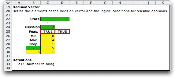
The decision is the amount of the opportunity in the portfolio.
We use  for
the investment amount. The decision is in cell C24. Cell
B29 controls an enumeration process that places the five
values of the decision variable in cell C24. Row 24 holds
logical expressions that determine whether a given decision
is feasible. for
the investment amount. The decision is in cell C24. Cell
B29 controls an enumeration process that places the five
values of the decision variable in cell C24. Row 24 holds
logical expressions that determine whether a given decision
is feasible.
|
Transition function |
The transition function
determines the next state, s', reached when decision d is
taken from state s. With two state variable, we
need two transition equations. The formulas for these equations
are in row 42.


|
Decision objective |
z(s, d), the measure of effectiveness
associated with decision d taken in state s.
For the investment problem, the return is taken from the
table of returns. the value of  determines
the column number and the value of determines
the column number and the value of  determines
the row number. On the Excel form this table value is transferred
by equation to cell F52. determines
the row number. On the Excel form this table value is transferred
by equation to cell F52.
z(s, d) =  |
| Recursive Equation |
The recursive
equation is the value of the optimum policy starting from
state s,  .
For a given decision made from state s, the
value of the portfolio .
For a given decision made from state s, the
value of the portfolio  plus
the value of the next state, plus
the value of the next state,  .
The recursive equation evaluates the maximum over all feasible
decisions. .
The recursive equation evaluates the maximum over all feasible
decisions.

In Excel the number in cell I53 is provided
by the computer as the value for the next state. Cell C52
is a formula that computes the sum of F52 and C52.

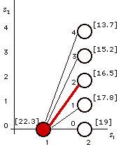
The figure below illustrates the computation
of the values given above.
|
Initial state set |
I = {s : states where the decision
process begins}
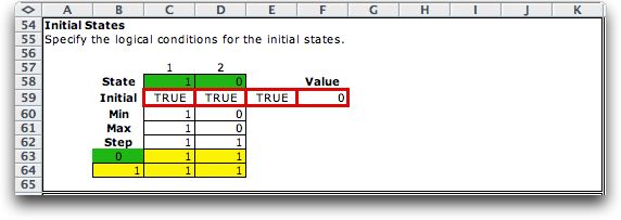
The investment example has only one initial state I =
(1,0). The Excel model identifies the initial states by
the Min and Max limits in columns C and D, and the logical
expressions in row 59. Cell E59 is True for an intial
state. The initial value function
is computed in F59. For the example it is 0.
|
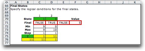
Final state set |
F = {s : states where the decision
process ends}
For the example the final state set is:  . .
The
Excel model identifies the final states by the Min
and Max limits in columns C and D, and the logical expressions
in row 71. Cell E71 is True for a feasible
state. The final value function,  ,
is computed in F71. ,
is computed in F71.
|
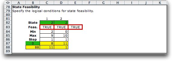
State space |
S = {s : s is feasible}
The Excel model identifies the feasible states by the
Min and Max limits in columns C and D, and the logical
expressions in row 83. Cell E83 is True for a feasible
state.
|
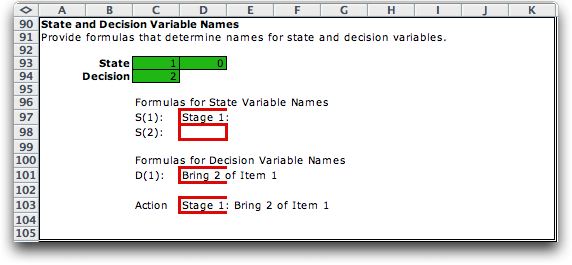
State and Decision Names |
This part of the worksheet is useful for output presentations.
Cells with red borders accept string expressions that provide
names for the states and decisions.
|
|
| |
|
|

