|
|
>  |
Teach
Dynamic Programming Add-in
|
 |
-
Line Partition
|
|
A class of problems for which dynamic
programming can be effectively applied involves the partitioning
of a line into non-overlapping segments. Applications include
production scheduling for finite time horizon, capacity expansion
of a production facility, and setting up inspection stations
along an assembly line. In the definition of these problems both
the state and decision vectors have a single component, making
them easy to solve. From a modeling point of view, they are illustrative
of the case where the classical stage representation for dynamic
programming is not appropriate. |
| |
Consider a line, as with n+1
discrete points or nodes numbered 0 to n.

The problem is to find an optimal partition
of the line into segments such that each segment begins at
one node and ends at another. Some objective or payoff
function is associated with each continuous subsequence of
nodes, and is typically nonlinear. The figure shows one
possible partition.

A
vector of selected nodes defines a solution, with each adjacent
pair of nodes defining a segment of the line. Thus a
general solution comprising k segments can be written
as a vector; that is,
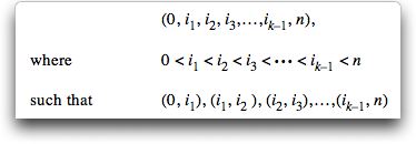
Note that
the number of segments, k, is a variable in this problem.
A
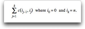
cost function is defined in terms of the nodes the comprise
the segments with c(i , j)
the cost of the segment starting at node i and terminating
at node j. The cost of a solution is the sum
of the segment costs. The goal is to minimize this cost.
|
| |
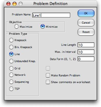 |
To make a model of this class, click the Line option
on the dialog. The line length is the number
of points in the line not including 0. Thus
when 10 is entered, the nodes on the line are
numbered 0 through 10.
The Max in interval entry is the
length of the maximum segment. In the figure
above, the center segment has a length of 4.
To reduce computation effort, this number might
be chosen as some number less than n.
There are three data form values 0, 1 and
2. We illustrate the three cases below.
|
|
Line Partition |
| |
 |
For this case we adopt a simple
cost function for a segment that is it is
the number of nodes in the segment squared
plus a fixed cost. For the example we use
a fixed cost of 10. Thus for a segment passing
from node i to node j the
cost is
c(i, j)
= 10 + (j - i)^2
The definition of this cost function distinguishes
one model from another. There are no restrictions,
such as convexity, on the characteristics
of the function. One of the strengths if
dynamic programming is that it can be used
for all kinds of objective functions.
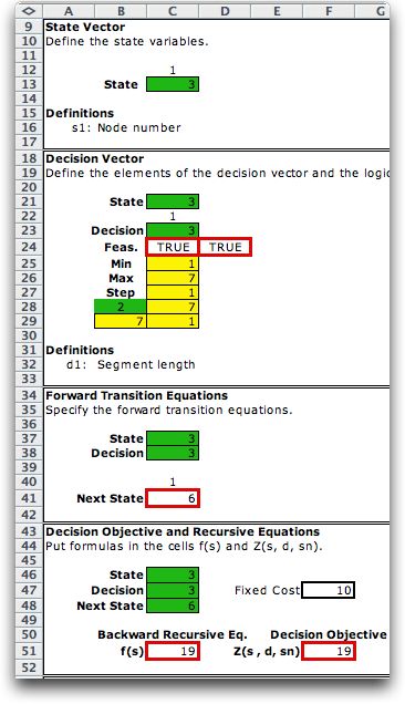
The model for this line problem is partially
shown at the left. The case illustrated is
for s=3
and d=
3. All
line problems have a single state variable
and a single decision variable. The maximum
decision value is set so that a segment does
not go beyond the last node.
The forward transition equation is:
s' = s + d
For the example s' =
6.
The add-in builds a worksheet
with all formulas and data structures automatically
provided. For some cases, the built in formulas
and data structure must be modified. In this
case the formula for the cost function is
placed in cell F51. The definition of the
fixed cost in F47 and the objective function
calculation in F51 is added to the model.
|
|
| |
Click the Solve button
at the top of the page to perform the dynamic programming algorithm.
For the example, we generate all feasible states first, and
then perform the backward recursion method of dynamic programming.
When the complete solution is obtained we use the forward recovery
method to return the solution. The solution is shown below
together with the statistics of the solution process.
|
Capacity Expansion |
| |
A power company expects a growth
in demand of one unit (100 megawatts) of power for each year
in the next 20 years. To cover the growth the company
will install additional plants with capacities in integer sizes
of 1 through 10. The size chosen will determine how many
years before the next capacity expansion is required. The
cost for the 10 sizes is shown below.
Size |
1 |
2 |
3 |
4 |
5 |
6 |
7 |
8 |
9 |
10 |
Facility Cost |
15 |
16 |
19 |
24 |
30 |
34 |
39 |
45 |
49 |
54 |
The goal is to minimize the present worth of the expansion
costs for the next 20 years. We use i to indicate
the interest rate for present worth calculations, and assume i =
5%. To illustrate how the objective function is evaluated,
say we choose to build plants in the size sequence 4, 6, 5,
5. This means that the expansions occur at times 0, 4,
10 and 15 so the present worth of the costs is

The situation can be modeled as a line partitioning problem
with

where c(d) is given in
the cost table as a function of the expansion size d. The
exponent of the discount factor is s, the year of
installation. In the DP model this is the state variable.
The problem is created in Excel with the Line option
on the model dialog. Here we specify the data structure option
as 1. The add-in builds the DP form and adds a single vector
to the right of the model (in column N). We have added the
entry in N9 to hold the interest rate. To complete the model,
place the function z(s, d) in cell
F51.
|
| |
Solving the problem yields the
optimum solution. A facility is built at time 0 of size 6.
The second facility is built at time 6 of size 6. At time 12
a facility of size 4 is built. Finally a facility of size 4
is built at time 16. The discounted cost of the plan is 83.73.
|
Production Scheduling (Wagner-Whitin algorithm) |
| |
A manufacturing facility has forecasted
demand for the next 20 weeks as shown in the table below. There
is a fixed cost for setting up a production run equal to f. In
addition, there is a variable cost v that is proportional
the number of items produced. If we produce more than
the demand in a particular week, the excess items are stored
until needed. The inventory cost is proportional to the
number of units and the number of weeks stored. The cost
per unit per week is w. The problem is to find
a production schedule that minimizes the total fixed, variable
and inventory costs. Demand data used for the example is below. |
Period |
1 |
2 |
3 |
4 |
5 |
6 |
7 |
8 |
9 |
10 |
Demand |
3 |
1 |
7 |
0 |
0 |
2 |
8 |
2 |
3 |
2 |
Period |
11 |
12 |
13 |
14 |
15 |
16 |
17 |
18 |
19 |
20 |
Demand |
9 |
4 |
1 |
8 |
3 |
3 |
8 |
6 |
5 |
5 |
|
| |
The appropriate dynamic programming
model is similar to that for the line partitioning problem. When
applied to the inventory problem, the approach is called the
Wagner-Whitin algorithm. The line to be partitioned in
this case is the time line. The nodes correspond to the
times {0, 1, 2,…,20}. A solution is described
by a sequenced set of times at which production occurs. For
this case n = 20. With the cost computations
described above, it can be shown that when production occurs,
it is always optimal to produce exactly the quantity demanded
for the interval being considered (Dreyfus and Law 1977).
To express the decision objective in general terms let  be
the demand in week t, and let c(s, s')
be the cost associated with producing at time s to
satisfy the demands for periods s+1 to s'. The
cost function has three components. be
the demand in week t, and let c(s, s')
be the cost associated with producing at time s to
satisfy the demands for periods s+1 to s'. The
cost function has three components.

To illustrate, we calculate z(s, s')
for s = 0, d = 6 and s' = 6. The
parameter values are f = 30, v = 4 and w =
1. 
|
| |
To implement the model in Excel, we again choose
the Line model option, but for this problem we use the Data
Form as option 2. This creates a two-dimensional table
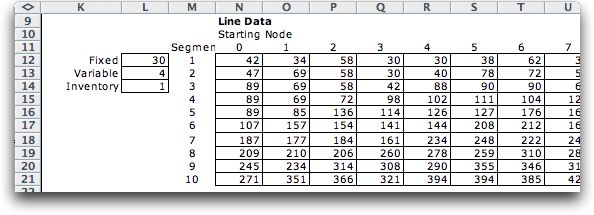
shown below as starting in column N. We have placed the cost
parameters in column L. Only part of the table is shown since
it has 20 columns. The table entries compute values for c(s, d),
the cost of producing items at time s. The amount
produced is sufficient to cover the demand for d periods.
For example the entry in cell N17, 107, is the cost of producing
13 units at time 0 and paying inventory on the items until
they are consumed.
|
| |
The Excel DP model requires no modification.
The decision objective formula is a direct reference to the
table.

|
| |
|
| |
|
The model requires a
state variable and a single decision variable.
Clicking the Solve button solves the problem.
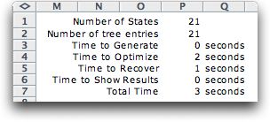
The solution statistics are below. There are 21
states.
Using the line partitioning model with this cost function,
the optimal sequence is (0, 6, 10, 13, 16, 20). The
table depicts the results. The first five components
of this sequence are production times; the corresponding
production quantities are 13, 15, 14, 14 and 24,
respectively. The total cost is 555. 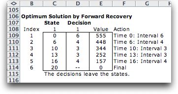
|
|
| |
If a problem is
equivalent to the optimum line partitioning problem,
DP requires only a single state variable. The problem is very
efficiently solved. |
| |
|
|

