|
|
>  |
Teach
Dynamic Programming Add-in
|
 |
|
|
|
Many operational problems in manufacturing,
service and distribution require the sequencing
of various types of activities or items. Examples
include a production facility in which chassis
must be sequenced through an assembly
line, an express mail service where parcels
and letters must be routed for delivery, and
a utility company that must schedule repair
work. In
this section, we introduce a robust dynamic
programming formulation that can be used
to tackle a number of such problems. In
most cases, however, the size of the state
space is an exponential function of the number
of items being sequenced.
To choose a sequencing problem select the Sequencing option
button on the Problem Definition dialog.
Choose a name for the model and specify whether
to maximize or minimize the objective. Specify
the number of items to be sequenced.
We discuss the data form option after the
model is described below.
|
|
| |
As a prototype, consider the problem of sequencing
a set of n jobs through a single machine that can
work on only one job at a time. Once a job is started,
it must be completed without preemption. The time required
to process job j once the machine begins to work on
it is p(j) for j = 1,...,n. The
associated cost c(j,t) is a function
of its completion time t and can take a variety of
forms, the simplest being
c(j,t) = a(j)t where a(j)
is the cost per unit time for job j. This form
admits a very simple solution when the objective is to minimize
the total completion cost of all the jobs. The optimum
is obtained by computing the ratio p(j)/a(j) for
each job and then sequencing them in order of increasing values
of this ratio. The job with the smallest ratio is processed
first, the job with next smallest ratio is processed second,
and so on until all jobs are completed. Ties may be broken
arbitrarily.
A much more
difficult problem results when each job j has a due
date b(j). The
cost of a job is zero if it is completed before its due date
but increases linearly if it is tardy. In our models, a(j)
is referred to as the penalty for a late job.

The goal of the optimization is to determine the sequence
that has the smallest total cost. The table gives
the relevant parameters for a 4-job instance.
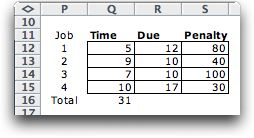
There are 4!
= 24 possible solutions. For the solution (3, 1, 2, 4),
the completion times are 7, 12, 21 and 31 respectively. Jobs
3 and 1 are completed before their due date so no cost is incurred. Job
2 is 11 days late resulting in a cost of $440 and job 4 is
14 days late resulting in a cost of $420. The total cost
is therefore $860. |
Returning to the Problem Definition Dialog |
| |
The problem definition dialog at the top of
this page has various options for specifying data forms for
the sequencing problem. When the Make Random Problem box
is checked, the random selects data to create interesting
problems. The DP model of the sequencing problem is
robust regarding the model for the objective function. We try
to illustrate this with the various data forms provided.
The data in the table for the example shows columns for time,
due date and penalty. The amount of data included in the table
depends on the Data
Form entry
on the problem definition dialog. The table above is data form
1. It assumes that the job penalty is constant with the number
of days late. If we had chosen data form 0, the penalty column
is not included. The jobs are assumed to have equal late
penalties of 1. With data form 2, a matrix is constructed
to show the late penalty as a function of the number of days
late. This would be useful when the late penalties are nonlinear
with time. The number of columns in this matrix is equal
to the total of the job times assigned during the generation
process. For the example that number is in cell Q15, so a
table with 31 columns would be constructed for data
form 2. If the number of columns is more than those available
on the worksheet, you will receive an error message.
The initial worksheet constructed depends on whether the Make
Random Problem box is checked on the dialog.
The Max Time entry provides an upper
bound to the job times when the Make Random Problem is
checked. With the default value of 10, all job times are
less than or equal to 10 as in the example. Using other maximum
time entries results in problems with greater time variety.
With the random option, due dates are are randomly selected
using the total job times as an upper bound. That sum
is calculated immediately below the time column. Even when
the Make Random Problem box is not checked,
the jobs are assigned random due times. Any numbers placed on the
data table by the add-in generation process can be replaced by
the user.
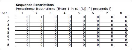
When the Sequence Restrictions box is checked, a table
is included on the worksheet to restrict the order of the sequence.
The table below shows a problem with eight jobs. The 1 in cell
(1,2) requires that job 2 precede job 1 in the sequence. Restrictions
such as these are easy to incorporate in the DP algorithm and
actually
make the problem
simpler.
|
DP Model |
| |
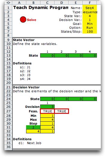 |
The add-in automatically creates
the model that solves the DP for a given number of jobs.
You can see the model by creating an example with the TeachDP
add-in or by looking at the example workbook for this section
(Worksheet Seq4 in teachdpdem.xls). The figure at the left
shows the state and decision vectors for the model
example.
The model requires a
state variable for each position in the sequence. The state
defines the set of jobs that are already scheduled. There
is a single decision variable that is the index of the
next job to schedule.
|
|
Solving the Problem |
| |
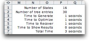
Clicking the Solve button
solves the problem. The solution statistics are below. The
program first generates the states. Since there are four binary
state variables, there are 16 states in the exhaustively generated
set.
The figure below shows the decision network for
the example. Each node represents a state. Each arc represents
a decision that leads from one state to another. Since a state
indicates the set of completed jobs, the finish time of the set
can computed as the sum of the job times for the jobs in the
set. Given the
state, the cost of adding a job to the set can be computed and
assigned to the decision arc. The DP solver has the problem of
finding the shortest path through the decision network from some
initial state to a final state. The heavy lines in the figure show
the arcs and nodes on the optimum path. The path starts at the
initial state
(0,0,0,0) and ends
at the
final state (1,1,1,1). |
| |
|
| |
The DP solution algorithm works
backwards starting from (1,1,1,1). It firsts finds the optimum
decision from each of the states with three 1's. These decisions
are trivial. For example, there is only one way to go from
(1,1,1,0), and that is J4. The cost
of J4 leading from (1,1,1,0) to (1,1,1,1) is 420. We assign
that value to state (1,1,1,0). Retreating to the states with
two 1 entries, there are two possible decisions. The optimization
finds the one that yields the smallest value. For example,
from state (1,0,1,0), J2 and J4 are the decisions. Given
the data the optimum is J2 with a cost of 440. It leads to
(1,1,1,0). Continuing with the states with only one entry with
value 1, each state has three decisions. All must be evaluated
to find the optimum at each state. For the example, we find
that from state (0,0,1,0) the optimum is J1. The cost associated
with that decision is 0 because J1 is completed on time. There
are four feasible decisions leading from (0,0,0,0). The optimum
is J3 leading to state (0,0,1,0).
At the completion of the solution process, we have for each
state the optimum decision and the optimum cost to reach the
final state. One last process is required. |
Recovering the Optimum |
| |
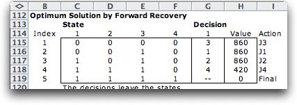
After the DP process is complete, we can find
the optimum from any state to the final state. Since we have
only one initial state, (0,0,0,0), we will find
the path from (0,0,0,0) to (1,1,1,1). The process is called recovering
the optimum.
State (0,0,0,0) has the optimum decision J3.
The value associated with (0,0,0,0) is 860, the length of
the path to (1,1,1,1). We record this as the first row of our
solution matrix. The decision leads to state (0,0,1,0), where
the optimum decision is J1 with cost of 860. It is the same
as (0,0,0,0) since the cost of J3 is 0. This leads to state
(1,0,1,0) where the value is again 860. Decision J2 with a
cost of 440 then leads to (1,1,1,0). The value at this state
is 420, the cost of the last decision J4. The last state has
no more decisions, so this is the final state. The optimum
sequence starting from the initial state is: J3, J1, J2 and
J4 with a total cost of 860.
The Options command under the Teach
DP menu allows various output alternatives to view the details
of the DP process.
|
Summary |
| |
Although DP is quite efficient for
small problems, the number of states grows exponentially with
the number of jobs. This 4 job example has 16 states, a five
job problem has 32 states, and in general the number of states
is 2 raised to the power of the number of jobs. |
| |
|
|

