|
|
To add a forecast, choose the Add Forecast command from
the Forecast menu. The dialog shown below is presented. The
field at the top shows the location on the worksheet of the
upper left corner of the forecast display. This option allows
an arbitrary placement of the forecast display and several
forecasts may be placed on the same worksheet.
|
| |
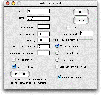 |
The Name field determines named ranges on
the worksheet. This name must be unique for different
forecasts. It must start with a letter and include no
spaces or punctuation.
The Data Columns field specifies the number
of individual time series that will be placed on the
display. It might be useful to have more than one if
the user has a several series to be simultaneously tracked
such as the stock prices in a portfolio or the sales
volumes for different products. Each time series will
have a separate forecast.
The Time Horizon is the number of
periods to be included in the series. This number can
be changed using the Change command. The History is
the number of periods of data used to obtain the first
forecast. All the methods require this warm-up period
to obtain valid forecasts. This history is important
because it limits several features of the forecast. For
instance the number of observations in a moving average
and the number of observations in a regression forecast
are limited to the number of periods in the history.
The forecast interval is also limited by the history.
|
|
| |
A nonzero entry in the Extra Data Columns field will
cause the add-in to create extra columns that are placed to
the left of the data columns. These might be useful for holding
associated information related to the data. For example on
the Investments page we
use a single extra data column to hold the dates associated
with closing stock prices.
A nonzero entry in the Extra Results Columns field
will cause the add-in to create extra columns in the display
that appear to the right of the forecasts. These might be useful
for additional processing of the forecasts. This is illustrated
on the Investments page
where we use several extra columns to make stock buy and sell
decisions.
When the Simulate button is checked, data will be
simulated using Monte Carlo simulation. The results are similar
to the Simulation command on the forecast menu, but
the data placed on the worksheet is fixed, rather than controllable
through simulation parameters.
When the Freeze Panes button is checked, the worksheet
window is divided into four sections and the panes are frozen.
This is useful for large data sets where the active data cells
may be far removed from the row and column titles.
The Seasonal button allows the analysis of time series
with cyclical variations. The number of data points in a cycle
is placed in the field below the button.
The Include Forecast button determines whether the
display will include forecasts for future times. For example
a moving average forecast places one column on the display
holding the moving average. When this button is checked, two
additional columns are also included, one holding forecasts
for future times and one holding error measurements for the
forecast. Usually one would check this button, but for some
applications future forecasts are not required. Again we illustrate
this on the Investments page.
The other pages of this section all include forecasts.
The dialog requires the selection of one of the forecasting
methods using the buttons on the right. In the remainder of
this page, we illustrate the various forecasting methods. |
Moving Average |
| |
|
Clicking the OK button causes the add-in to construct
the form shown at the left. Cell C3 gives the name of the
data. This cell should not be changed. Cell D4 contains
the number of data points to be included in the moving
average. This number can be changed to observe the effects
of different lengths. It can be no greater than the history,
10 in this case.
The data is in column C. Cells C10 through C19 hold data
for the warm-up period. For a moving average of 10, there
must be at least 10 data points available for the first
forecast. The data shown is a simulated random variable
with a mean of 50 and a standard deviation of 5. Column
D holds the estimate of the mean of the time series. The
moving average estimates only the mean. Column E shows
the forecast. The time interval, t, for the estimate
is set in E4 by the user. For the example t is
2. The number can be changed but is limited from above
by the history. The entries in column E are offset by t periods
from the moving average value from which the forecast was
derived. For example, the entry in E21 is the forecast
for time 2 based on the moving average computed for time
0 in cell D19. The two values are equal because the moving
average assumes a constant for the underlying mean value
of the time series. The column is labeled Fore(2) to indicate
that it holds an estimate of the time series based on the
mean value estimated two periods earlier. |
|
| |
Column F computes
the forecast errors. The error is simply the difference between
the value observed for a period and the forecasted value. For
example, the entry for period 2 which appears in cell F21 is
the value of the data in period 2 (cell C21) less the value
of the forecast (cell E21).
The means and standard deviations of the columns are computed
in rows 6 and 7. The moving average column should have less
variability than the data column because moving average eliminates
some of the noise variability. The error column variability
depends on both the data variability and the variability of
the forecasts.
Row 8 (cell F8) shows the MAD or Mean absolute deviation of
the error results. This is sometimes used as a measure of forecast
quality.
In practice, one would fill in a table like this one period
at a time as data is observed. Data not yet available are indicated
by ***, as shown for periods 16 through 20. Moving averages
are computed for these periods because the moving average function
looks back the specified number of periods (10) and uses as
many numeric values as available. For example, the moving average
for period 20 (in cell D39) is the average of the five data
points for periods 11 through 15. |
| |
|
The selection of the number to be included in the moving
average is the prerogative of the analyst. If the mean
of the underlying time series is truly constant, the average
should be as long as possible. In reality the mean value
may be changing. If the forecast is to discover changes
quickly, the number in the average should be low.
The same series is shown at the left with 5 periods in
the moving average. The standard deviation of the forecast
has increased because the noise has more effect because
of the smaller number of periods in the average. |
|
Exponential Smoothing |
| |
|
The display at the left shows the same data with forecasts
provided by the exponential smoothing method.
This method has a single parameter Alpha. A small
value of Alpha tracks rapidly varying time series
better than a large value, but a small value is more affected
by noise. The value of Alpha for the example is
in cell J4. The default value is
2/(history + 1)
Alpha can be changed by the user.
The forecast for time 0 (cell J19) is computed by a moving
average with length equal to the history (10 in this case).
Exponential smoothing requires such an estimate to get
started.
The time interval of the estimate is in K4. The estimates
for the mean of the series are in column J and the forecasts
are in column K. Since exponential smoothing only estimates
the mean, the forecast will be the same as the estimate t periods
earlier. |
|
Regression |
| |
|
The regression method is similar to the moving average
method in that it uses a fixed interval to determine forecasts.
The example uses 10 periods. The method takes the last
10 observations and constructs a linear regression estimate
for the mean of the time series. There are two results
of the regression, a constant term labeled Reg. a, and
a linear term labeled Reg. b. Estimates are computed with
the linear expression:
Est(t) = a + bt
where t is the interval between
the time of the estimation and the estimated mean value.
For example, the estimate for time 4 (cell R23) is based
on the regression coefficients computed at time 3 (cells
P21 and Q21). With all values rounded to two decimal places,
this is
Est(2) = 49.95 + (0.22)(2) = 50.40
The numbers used by Excel have many significant
digits of accuracy, but when rounded values are shown the
results seem to have small errors. For the example we would
expect 50.39 as the result, but actually the value 50.40
is more accurate.
The data observed for time 4 (cell O23) is:
38.03, so the error for time 4 (cell S23) is
38.30 - 50.40 = -12.11
The regression method is useful for time
series that have a trend component. Again the choice of
the length parameter is important. For rapidly changing
series the length should be short. For slowly changing
series that can include a trend the length should be long.
The value of the length can be changed in cell P4, but
it cannot exceed the history. |
|
Exponential Smoothing with Trend |
| |
|
This method is also used when the series might have a trend.
It is similar to the exponential method, but also estimates
the value of the trend component. Like the regression method,
both the constant term and the trend are estimated. It has
two parameters, Alpha and Beta. The estimates
for time 0 are obtained with a regression forecast. |
|
More than One Forecast |
| |
|
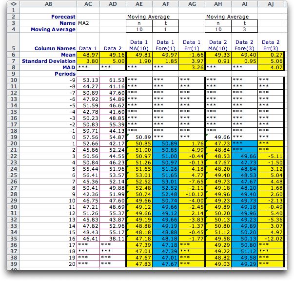
The Add Forecast dialog allows for the analysis
of more than one series . The dialog is shown below for
two series.
The forecast is produced below using simulated
data. Both forecasts use the same method but may have different
parameters. |
|
Seasonal |
| |
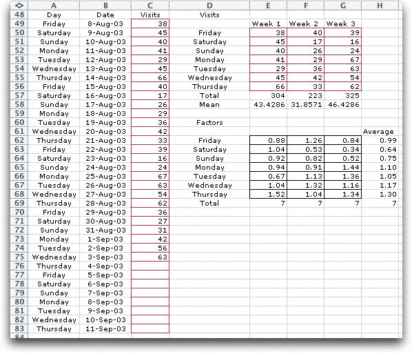
To illustrate the
use of the Seasonal button, we consider a time series
that observe the visits to a web page. Data showing the visits
to the site for a 28 day period is shown below. It appears
that there is a weekly variation in the data with the fewest
visits on Saturday and Sunday. We have tabulated the first
three weeks at the top right with the total and average number
of visits per day. At the bottom right we divide the visits
by the average for each week to compute the relative number
of visits compared to the average. Finally we average these
over the three weeks to compute an adjustment factor for the
days.
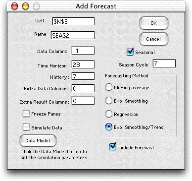
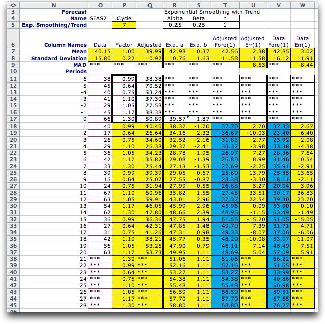
To analyze the data we click the Seasonal button
on the Add Forecast dialog and indicate the Season
Cycle as 7. One week is specified as the history and we
provide room for 28 days of data.
The forecast is produced below with the data
placed in column O. Column P is for the adjustment factors.
The first 7 cells in this column hold the factors computed
above. The remaining cells in this column hold equations linking
to the first cells. Thus changing the factors in the first
7 cells will change the entire column. The adjusted data is
computed in column Q by dividing the data by the adjustment
factors. Columns R and S perform the exponential smoothing
with trend to forecast the adjusted data in column T. The forecasted
visits in column V are computed by multiplying column T by
the adjustment factors.
|
| |
|


