| |
 |
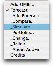
The Simulate option is for the comparison of different
forecasting methods on a single time series using simulated data.
The process is similar to the Compare option, but here the simulation
is live in that the model parameters can be changed on the worksheet
and the series and forecasts are automatically adjusted. The option
is useful to illustrate the impact of trends, steps and noise
on forecasts and their accuracy.
|
| |
|
The dialog allows selection of a name, time horizon, history
and number of extra columns. The check boxes at the bottom
select one or more forecasting methods. The fields to the
right of the check boxes indicate how many forecasts of each
type are to placed on the worksheet. |
|
| |
Clicking the data
model button presents the Model Data dialog. Here we set the
initial parameters of the simulated model. The same button
appears on the other options for setting the parameters of
the simulated data. In addition to determining the integrality
and nonnegativity of the data, the option allows the user to
introduce random changes in trend and random steps in the base
of the time series. For both steps and trends the probability
specified determines the chance that a change will occur at
any given period. The mean and standard deviation of the magnitude
of the change, if it occurs, is also given here. The Base SD
is the standard deviation of the noise added to the model.
The parameters are used with Monte Carlo simulation to determine
the time series. The model assumes that change and noise values
are governed by Normal distributions. |
| |
|
The simulation requires a number of additional columns
on the worksheet. The Hide Simulation button allows
these columns to be hidden. The particular model simulated
here has an initial trend of 1, but no step or trend changes. |
|
| |
 |
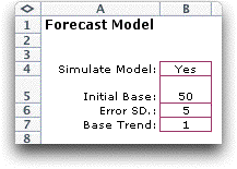
On clicking OK a worksheet is created with the same
name as the forecast. The simulation parameters are placed
in the corner of the worksheet. Changing any parameter
changes the simulated series.
The columns showing the simulation are shown below. One
or more columns of random numbers appear first. The example
is affected by only noise so only column F is necessary.
The numbers in cells F11 through F40 are simulated from
a uniform distribution with range 0 through 1. The numbers
are controlled by a seed appearing in cell F9. The simulation
can be regenerated by using the Fill Down option
on the Change menu item. |
|
| |
Columns G though J
hold the base, trend and cumulative trend. The cumulative trend
is added to the base to determine the mean value for the model.
The Noise in column K is simulated with the Monte
Carlo method using the random numbers in row F. The noise values
are drawn from a Normal distribution with mean 0 and standard
deviation 5. The standard deviation is stored in cell B6.
The value of the time series is the sum of the model and the
noise. For the example we round this sum to the nearest integer. |
| |
|
| |
In the example, we use
both an exponential forecast and an exponential forecast with
trend. First consider the exponential smoothing results. With
simulation, we know both the series value and the model. Column
O holds the one period forecast error comparing the observation
in one period with the forecast in the previous period. Note
that the standard deviation of the error is approximately the
noise standard deviation. The error has a positive bias because
exponential smoothing estimates always lag for a series with
a positive trend. The model error computes the difference between
the model and the estimate from the previous period. The bias
in the model error is about the same, but the standard deviation
is much lower because the error does not include the noise variation
of the observation. |
| |
|
| |
When we include the trend
estimate, the bias for both observation errors and model errors
is much smaller. Again we note the smaller standard deviation
for the model errors. Although this example shows a negative
bias, the bias should tend toward zero as more observations are
included. With the chosen values of alpha and beta, the initial
estimate of the trend is reflected throughout the 20 period time
horizon. |
| |
|
To illustrate a more complicated simulation, we create
a second model with both step and trend changes. The model
dialog is at the left. |
|
| |
|
|
The parameters are on the left and the simulated time
series is shown below. We note two step changes in the
first three periods and four trend changes in 30 periods
of the analysis. It is useful to simulate complicated time
series to observe the response of forecast methods to various
kinds of changes.
Changing the parameters or the random number seeds, results
in a different simulated time series. |
|
| |
|
| |
|


