|
|
 |
Forecasting |
 |
-
Functions |
|
|
|
Many of the
computations for the Forecasting Add-in are accomplished by functions
provided by the add-in. The functions are automatically inserted
into the forecasting forms. They can also be used independently
in worksheet formulas. They are
found in the Excel function list under the heading User Defined
Functions. The function names all have the FF_ prefix. They
are listed below with their arguments. Some of the functions have
range arguments. We show images of forecasts of the various kinds
to discuss the functions and their purposes. In some cases
the activities of the functions could have been carried out with
normal Excel functions or calculations. We use functions so that
missing or non-numeric data will return the text string ***. This
allows the forecasting to continue even when some data is missing.
It is important to remember that user
defined functions are linked to the add-in that created them.
For example, all the function references in the Forecast demonstration
workbook are linked to the add-in in the computer where they
were created. When opened on another computer the reference
includes a path to that add-in. Since obviously the user cannot
open that author's add-in, the reference must be adjusted to
link to the copy of the Forecast add-in on the user's hard drive.
We provide the Relink command on the Forecast menu to fix some
of the references. In particular, any worksheet formula that
uses the function as the first entry after the "="
sign will be corrected. Every function used by the add-in is
placed first in the formula, so all of these references are
corrected by the Relink command.
If the user places a function within
a cell formula, the reference will not be corrected. All such
links can be redirected by the more general Excel Links
command on the Excel Edit menu. |
Functions used by Moving Averages |
| |
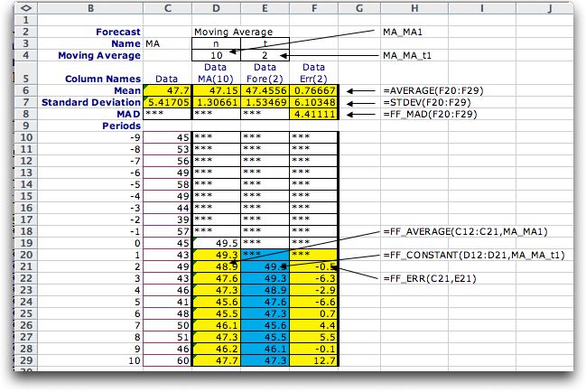
The functions refer
to two named cells at the top of the display. The length of
the moving average is stored in cell D4 with the name MA_MA1.
The forecast interval is stored in cell E4 with the name MA_MA_t1.
The prefix to the names is the name of the forecast. The figure
below shows the function references used on the worksheet.
The functions are described under the figure.
|
| |
| AVERAGE(F20:F29)STDEV(F20:F29) |
This Excel function is placed in row 6
for each display column. It computes the mean of the entries
in the columns below. Note that the range for the mean
values does not include the warm-up period whose length
is the history. The history value is 10 for the
example. |
| STDEV(F20:F29) |
| This Excel function is placed in row 7 for
each display column. It computes the standard deviation of
the entries in the columns. Again only the data values starting
at observation 1 are considered. At least two numeric values
must appear in the column for a numeric result. |
| FF_MAD(F20:F29) |
| This function computes the mean absolute deviation
of the numbers in a range. The absolute value of each number
in the range is computed and the average of these values
is returned as the result. This is an interesting measure
for forecasting errors because it is increased by the absolute
value of both the mean and variation about the mean of the
errors. The FF_MAD function is only used for error columns. |
| FF_Average(C12:C21,MA_MA1) |
This function computes the moving average.
It has two arguments: a range and the number of values
to be used for the moving average, or the moving average
interval. The number of elements in the range must be at
least as great than the number in the moving average. For
the example, the range has 10 elements and the number in
the average is also 10, so the example computes the average
of the 10 numbers in the range (C12:C21). The function
is useful because it allows experimentation over different
values of the moving average interval. Only numeric values
in the range are used in the average with blanks or strings
contributing to neither the numerator or denominator of
the average. At least one cell in the averaged range must
contain a number. Otherwise the function returns "***".
The example shows the function in row 21. The function
is repeated in rows 20 through 29 with adjusted range references.
This is also true for the other functions described below. |
| FF_CONSTANT(D12:D21,MA_MA_t1) |
This function creates a forecast from a
model that assumes that the time series varies about a
constant mean. It's range covers the moving averages for
10 periods. The second argument indicates the time interval
for the forecast. The value for the interval for the example
is 2 indicating that the forecast is the moving average
value computed two periods earlier. Thus the result for
the example in cell E21 come from the moving average computed
in cell D19. The value of the time interval may be changed. |
| FF_ERR(C21,E21) |
| This function computes the difference between
an observation and a forecast. For the example it computes
the difference between the entry in C21 and the entry in
E21. |
|
Functions used by Exponential Smoothing |
| |
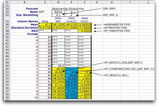
The figure below shows
the function references used on the worksheet for exponential
smoothing. The functions refer to two named cells at the top
of the display. The value of the Alpha parameter is
stored in cell D34 with the name EXP_EXP1. The forecast interval
is stored in cell E34 with the name EXP_EXP_t1. The prefix to
the name in each case is the name of the forecast. Only the FF_EXP
function is different than those used for the moving average.
It is described under the figure.
|
| |
| FF_EXP(C51,D50,EXP_EXP1) |
This function computes the exponential
smoothing estimate of the time series mean value. It has
three arguments, the current data, the previous estimate
and the value of alpha. For the example in cell D51 these
values appear in cells C51, D50 and EXP_EXP1. |
|
Functions used by Regression |
| |
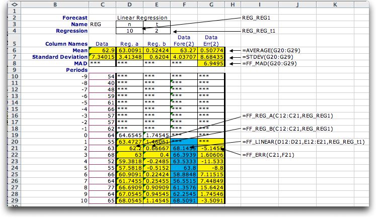
The figure below shows
the function references used on the worksheet for regression
forecasting. The functions refer to two named cells at the
top of the display. The value of the number of points to be
used in the regression is stored in cell D4 with the name REG_REG1.
The forecast interval is stored in cell E4 with the name REG_REG_t1.
The prefix to the name in each case is the name of the forecast.
The example is simulated from a model with an initial trend
of 1.
|
| |
| FF_REG_A(C12:C21,REG_REG1) |
This function is
used to compute the constant value of a linear regression
equation. The range argument contains the dependent values
used to fit the regression line. Only a specified number
of elements in the range are used. This regression interval
is given as the second argument. For the example, the
range has 10 elements and the number in the regression
is also 10. The independent values for the equation are
the time indices immediately preceding the cell in which
the value is computed. The example computes the
regression constant at time 2. The variable regression
interval is useful for forecasting because it
allows experimentation over different values. The function
is used for regression forecasting. Only numeric values
in the range are used with blanks or strings not contributing
to the result. At least two cells in the range must contain
a number. Otherwise the function returns "***". |
| FF_REG_B(C12:C21,REG_REG1) |
This function is
used to compute the trend value of a linear regression
equation. The arguments are the same as used for computing
the constant term. |
| FF_LINEAR(D12:D21,E12:E21,REG_REG_t1) |
This function is used to make
forecasts with linear models. The first two arguments are
the ranges of the constant and trend estimates respectively.
The third argument is the time interval for the forecast.
The function retrieves the values of A and B computed t periods
earlier and computes.
A + Bt
The example in cell F21 uses the constant and trend values
computed in D19 and E19 respectively. The function returns
"***" if any of its arguments are not numeric. |
|
| |
Functions used by Exponential Smoothing with Trend |
| |
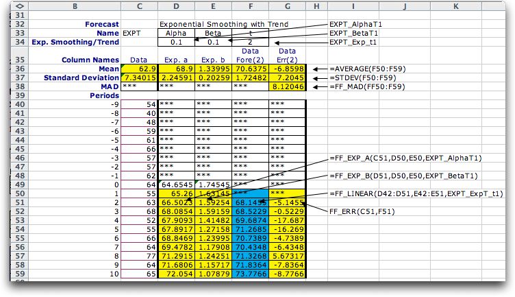
The figure below shows
the function references used on the worksheet for exponential
smoothing with a trend forecasting. Another name for this is
double exponential smoothing. The value of the Alpha parameter
is stored in cell D34 with the name EXPT_AphaT1. The value
of the Beta parameter is stored in cell E34 with the
name EXPT_BetaT1. The forecast interval is stored in cell F34
with the name EXPT_Exp_t1. The prefix to the name in each case
is the name of the forecast. The functions unique to this method
are described below the figure.
|
| |
| FF_EXP_A(C51,D50,E50,EXPT_AlphaT1) |
To compute the current estimate of the
mean of the time series this method uses the current observation,
the previous constant estimate, the previous trend estimate
and the parameter alpha. These are the four arguments
of the function. The value returned is the constant value
of the linear equation that will provide the forecast.
If the data argument is missing,
the function provides an estimate based on the other
parameters. When other arguments are missing
or not numeric, the function returns "***". |
| FF_EXP_B(D51,D50,E50,EXPT_BetaT1) |
This function is
used to compute the trend value of the linear equation
based on the current and previous estimates of the constant
term, the previous estimate of the trend and the parameter beta.
These are the arguments of the function. |
|
| |
Functions used by Simulation |
| |
Several functions
are used for simulating a time series as illustrated in the
figure below. The simulation parameters are placed in a parameter
range shown in B8 through B15. Changing numbers in this range
changes the simulated results.
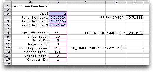
|
| |
| FF_RAND(seed) |
This function returns a random
number drawn from a uniform distribution with range 0
to 1. The function uses the internal Excel random number
generator. The value of the function depends on the seed.
We use this function in the forecast simulations by having
the random number for one period be the seed for the
next. Then by specifying the first seed, the complete
sequence of random values is determined. This is handy
so the same sequence of random numbers can be used in
different simulation experiments. The example is illustrated
in cells B4 through B6. The seed value in B3 controls
the three random values that appear below it. Each call
of FF_RAND uses the previous value as its seed. |
| FF_SimErr(prob, parameter
range) |
This function is used to simulate
the noise of a simulated time series. The function assumes
that the noise is Normally distributed with 0 mean. The
standard deviation of the noise is the third cell in
the simulation parameter range. For the example, this
is in cell B10. The Monte Carlo method provides the simulated
value. The prob argument is a uniformly distributed
random variable provided by the FF_RAND function. The
example in cell E8 computes the simulated value from
the random number in B4. |
| FF_SimChange(probchg,
probvalue, parameter range) |
This function computes either trend changes or step
changes in the simulated series. For both, there is a specified
probability that a change will occur (0.1) for the example
below. If it does occur there is a specified mean (0) and
standard deviation (1) of the amount of the change. Two
random numbers are required to evaluate the function. The
argument probchg is the random number determining
if a change does occur. If this random number is less than
the probability of change, the change occurs.
If the change occurs, the second random number, probvalue,
is relevant. It then determines the magnitude of the
change. The probability of change, the mean value of
the change and the standard deviation of the change are
provided by the parameter range. For the example in cell
E12, the random number in B5 is more than the change
probability, so no change is experienced. Thus, we see
the value of 0 in E12. |
|
| |
Other Functions |
| |
Two other functions are
used in forecasts that involve seasonality and portfolios. |
| |
| FF_ADJUST(factor1, factor2) |
This function simply
multiplies factor1 by factor2. It is used in for forecasts
involving seasonality. We use this function rather than
simply multiplying the two numbers together because the
function returns the text string *** when one of its
arguments is not numeric rather than an error indication. |
| FF_SUMPRODUCT(range
1, range 2, interval 1, interval 2, start 1, start 2) |
This function is does the same
as the Excel SUMPRODUCT function except on different
size ranges. Elements of the two ranges are in range
1 and range 2. The numbers in range 1 to
be summed are in columns that differ by interval
1. The numbers in range 2 which are to be multiplied
by the numbers in range 1 are in columns that differ
by interval 2. The arguments start 1 and start
2 indicate which elements are to be summed. Examples
are below when range 1 = (1, 2, 3, 4,
5, 6) and range 2 = (1, 2, 3, 4)
FF_SUMPRODUCT((1, 2, 3,
4, 5, 6),(1, 2, 3, 4),3, 2, 1, 1) = 1*1 + 4*3 = 14
FF_SUMPRODUCT((1, 2, 3, 4,
5, 6),(1, 2, 3, 4),3, 2, 2, 2) =2*2 + 5*4 = 24
FF_SUMPRODUCT((1, 2, 3, 4,
5, 6),(1, 2, 3, 4),3, 2, 3, 1) = 3*1 + 6*3 = 21
The function is used in Portfolio forecasts. |
|
| |
|
|


