 |
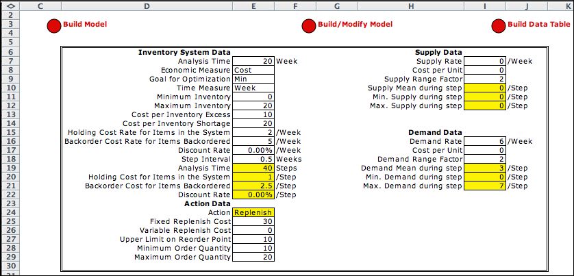
The data below shows the
parameters of our example problem. Note that the supply rate
is specified as zero while the demand rate is 6. This is typical
of inventories where product is withdrawn at random times and
replenished when necessary. The costs of demand and supply
are both zero. The total cost used by the analysis
is an estimate of the inventory operating cost.

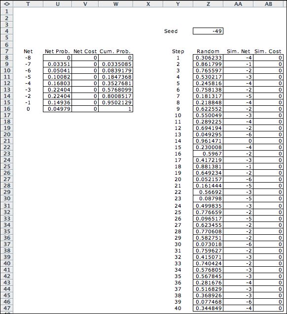
The distribution of the demand is shown in columns U and V.
The random variables are negative indicating that demand draws
material out of the inventory. The deterministic model uses
net demand simulated from this distribution. The simulated
values are linked to a random number seed entered in cell Z5.
A different simulated sequence is obtained with a different
seed.

|
| |
The demand expressed as positive
quantities is shown in the chart below. The deterministic DP
problem is to find a sequence of replenishments to meet this
demand that minimizes total cost. |

|
|
| |
We create the model by clicking the Build
Model button at the top of the data worksheet. A new worksheet
is created with the name DDP_Model. The DDP has only
states and actions. For the DDP demand is not a random
variable but a simulated value for each of the 40 steps of
the analysis.
The model has two state variables, the first is the step number
(time). The second state variable (stock) is the inventory
level. Cells with yellow color and red outlines hold formulas
linking the cell contents to entries on the data worksheet.
In particular the maximum for state variables are linked to
the corresponding values on the data form. The cost coefficient
for stock (G21) has a formula that evaluates as the unit holding
cost when the stock level is positive and the negative of the
unit backorder cost when the stock level is negative.
The action variable has two dimensions. The first indicates
whether a replenishment order is placed, and the second is the
amount of the replenishment (lot size). The logical condition
in K17 returns FALSE when the replication variable is 0 and
the lot size is greater than 0. |
| |

State subsets are included in the model to
identify the terminal states. All states with time equal
to 41 exit to the final state.

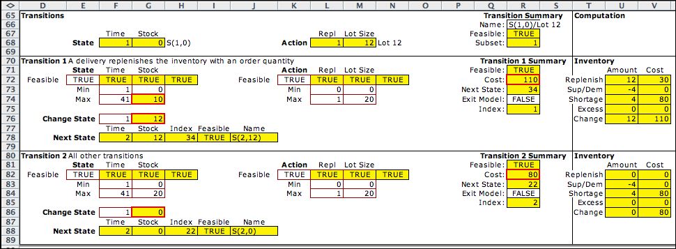
A decision is the combination of a state and
an action. The decision subsets limit feasible combinations.
The bounds of Decision 1, allow orders when the stock
is at or below the reorder point. The order size is limited
between the minimum and maximum lot size. The current state,
(1,0), and action,
(1,12), satisfy these requirements.

The transitions for the DDP compute the next
state given the current state and action. Computations unique
to the inventory problem are performed in columns T through
V. The numbers computed there give the Change State vector
and the Cost for each decision.

|
Enumeration |
| |
Clicking the List Elements button
at the top of the model worksheet causes the program to sequence
through all feasible states. The resultant list has 862 entries.
The last state is the Final state.

...

The action list has the Hold action that indicates
that the replenishment quantity is 0. The other actions prescribe
replenishment amounts between 10 and 20.

|
Decisions |
| |
For the DDP problem, feasible
decisions and transitions are shown in the Decision List.
A decision is described by a state and an action. The first
25 decisions are shown below.

...

There are 5702 decisions for this model. The decisions for
step 41 all go to the Final state. The final state
has a null transition. |
Call Solver |
| |
The DDP model uses the DP
Solver to find solutions. The Transition structure available
for the DDP is the Transition List. A different name
can be specified other than the one provided.

Part of the DP Solver worksheet is shown
below before optimization.
|
|
| |
Clicking the Solve button
presents the iteration dialog. The Acyclic option
is best for this problem since the state transitions always
go to a state with a greater index. The single
exception is the final state that has a self loop. The Acyclic
option solves the problem in a single pass through the states
from bottom to top.

At the completion of the computation, the solver model has the
solution shown in columns K through L. The optimum action
for each of the 862 states has been determined. The results comprise
the optimum policy.
|
|
| |
For a deterministic problem, the
solution can be traced from an initial state to the final state.
To find the optimum, click the Recover Optimum button.
Choose the intial state index. For the example we choose state
1. S(1,0). Clicking OK constructs the list of states on the
optimum path from the initial state. The list is placed just
below the state
list. Starting from state 1, the optimum
sequence of states with their corresponding actions is shown
below. |
| |
|
| |
The chart of the inventory levels
is below.

Because the lead time is 1 step, the first step
has lost sales of 4. After that the replenishment quantities
always satisfy all demand. Every order replenishes the sum
of some number of steps into the future. For example the 12
units delivered at the end of step 1 satisfies the requirements
of periods 2 through 6. |
Summary |
| |
The complexity of the deterministic problem
depends on the numbers of states and decisions.
For this model, the number of states is equal to the number
of steps in the time horizon multiplied by the number of integers
in the range between minimum and maximum inventories. If either
of these numbers is large, the number of states is also very
large. The number of decisions is always greater
than the number of states.
|
| |
|


