|
|
 |
Dynamic
Programming
Data |
 |
-
Inventory |
|
Inventory systems are important
in many aspects of modern life. The kitchen pantry, refrigerator
and freezer are the repositories of inventories where food
items are purchased in package size and
consumed over a period of time. When the amount of the
food item is depleted or reaches some low level, the inventory
is replenished with a trip to the market. It may be less expensive
to purchase and store amounts greater than necessary for immediate
consumption. Often a larger package has a smaller unit product
cost than a smaller one. Also buying larger amounts requires
fewer trips to the market. On the negative side, a larger package
requires a greater investment of capital and there is commensurate
cost of the invested capital. Of course there are many other
issues of sometimes primary importance such as
the cost of the storage space, the risk of spoilage for food,
and the possibility of obsolescence for other material goods.
Inventories of other stored quantities are primary concerns
in many areas of business and government. In factories, parts
are often produced in lots of many units so the cost of
setting up the production process can be spread over the
units of the production lot. Raw materials are often delivered
in lots of more than one unit, but used over a period of time.
Water reservoirs are inventories of water
that are replenished through precipitation runoff or importation
and depleted by water releases, demand, or evaporation. Facilities
are sometimes built larger than immediately necessary to take
advantage of economies of scale. The unused capacity can be
thought of as inventory. People waiting for a service such
as a subway train can be viewed as an inventory that grows
through arrivals of travelers and depletes when a train
arrives, fills and departs.
The control of inventories is an aspect
of operations management and is covered in many books on the
subject. This web site has at least three major sections that
deal with inventory. The Inventory
Theory section provides the derivations of formulas
for computing the optimum lot size for deterministic abstractions
of inventory models. The Inventory
Add-in provides numerical solutions for several models
involving both deterministic and stochastic demand. The Inventory
Game is a template that allows students to make real
time decisions about the control of a single product inventory.
The cost of inventory is included in many mathematical programming
models of applied problems.
This section describes dynamic programming models of a single
product inventory system. We consider four kinds of models:
deterministic DP, Markov decision process, discrete time Markov
chain, and continuous time Markov chain models. |
Creating a Data Form |
| |
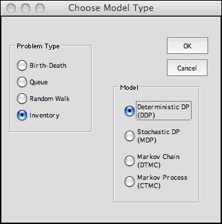
To get started, select the Data command
from the DP Data add-in menu. Our first illustration
is for the deterministic inventory system (DDP). Choosing OK
presents the dialog for naming the problem and choosing to
replenish or purge. The problem name must consist of all letters
with no punctuation except the underline symbol.
|
| |
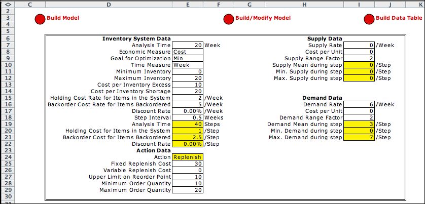
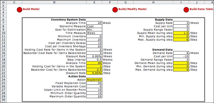
The data page shown below is constructed.
All white cells can be changed, but the yellow cells should not.
Changes in the model parameters are reflected directly on the
model worksheet. The Build Model button calls
the DP Models add-in to automatically construct the
model. The Build/Modify Model button also builds the
model but first presents a dialog allowing model parameters to
be changed. This is useful when the student wants to change the
model in some way. The Build Data Table button constructs
a data table that computes necessary probability distributions.
It is discussed near the bottom of this page. |
| |
|
The Inventory |
| |
The figure shows
an example of the inventory pattern assumed in the models of
this section. The level of the inventory, I, indicates
the amount of material on hand or the amount backordered. Time
is measured in steps, labeled below as 0, 1, 2 ... . For purposes
of analysis, the inventory is constant for the duration of
steps, but varies from one step to another because of supplies
that add material, demands that remove material, replenishments
that increase the inventory in lots, and purges that
decrease inventory in lots. A lot is an amount of the product
that is either added or removed from the inventory at discrete
times. In this discussion we consider
an inventory system primarily affected by demand with inventory
replenished in lot size amounts. We consider
the purge option later.

|
| |
|
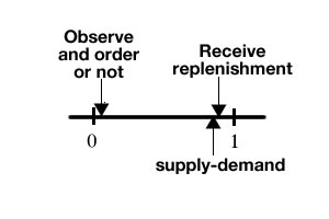
When modeling the system
it is important to identify the exact moments in time when
important activities happen. The model we construct assumes
that at the beginning of each time step the inventory level
is observed. At that time a decision is made to order a
replenishment or not. The size of the replenishment lot
is also specified. Near the end of the interval the inventory
is changed by adding supplies and subtracting demands that
occur within the interval. After this, but just before
the beginning of the next interval the replenishment order
is received. When the next step begins, the inventory is
adjusted to account for the supply, demand and replenishment.
The figure shows the sequence of events. In fact the actual
timing of all events is at the step boundaries, shown as
0, 1, 2 ..., but the sequence of the events is as explained.
The effect is that the system has a lead time for replenishment
of one step duration.
|
|
| |
The equations that
govern the sequence of inventory levels would be simple if
there was not the possibility of the inventory falling below
the minimum inventory or above the maximum inventory. Both
of these eventualities are penalized in our model and the inventory
level does not venture beyond these extremes at any time.
The sequence of events shown above indicates that the lowest
inventory level during a given step occurs right after the
demand for the step has been withdrawn. If the inventory falls
below the minimum there is a shortage in inventory as computed
below. The maximum inventory level in a step is just after
the replenishment has been received. If the level is greater
than the maximum the result is the excess inventory as computed
below. The transition function computes the new inventory level.
The equations below describe a system that has a lead
time of one step. Any replenishment ordered at the beginning
of the step is not available to meet the demand during the
step. It is available to meet the demand of the next step.
The equations use the net supply, w. This will be
a negative random variable when the demand is the primary driver
of the inventory level. The replenishment amount, q,
is a decision variable in our models. It may be zero for some
steps and positive for others.
|
| |
|
Some of the parameters used
in the notation above are entered in the system data form.
The first entry shows the time horizon for the deterministic
problem. The next entry indicates the economic measure.
The optimization goal shows the direction sought by optimization.
The time measure is in the fourth row. The minimum and
maximum inventory levels are next. Then comes a variety
of cost parameters. Finally the discount rate per unit
time and the step interval are entered. We use a discount
rate of 0% in order to minimize the total cost of operating
the inventory.
The following yellow cells compute the step
parameters used in the analysis. The step size of 0.5
results in an analysis horizon of 40 steps.
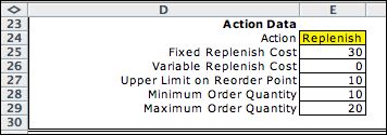
The action data provides fixed and variable
costs for replenishment. The fixed cost is experienced
only when the replenishment amount is nonzero.
The following describes the computation of
total cost per step. |
|
Actions |
| |
Two kinds of actions possible with these models.
The Replenish action means to add inventory in some
nonzero amount called the lot size. The alternative is the Purge action.
This action removes some nonzero amount, again called the lot
size. A replenish action is appropriate for product inventories
provided to fulfill customer demands for receiving the product.
The purge option is for inventories such as a batch process.
Here units of product gather into an inventory waiting for processing.
At some time the process removes a batch from the inventory for
processing. |
| |
|
Cell E24 indicates the action
type specified for the model. It is colored yellow to indicate
that the model structure determines for the form of the
model. Once the model is constructed it cannot be
modified to represent the alterantive action.
|
|
|
| |
The model treats supply and demand
as random variables governed by the Poisson distribution. The
parameters of the supply and demand are in column I in the data
below. The values are different than the parameters we use for
our example, but they will serve to illustrate how the model
handles the supply and demand random variables. |
| |
|
| |
Supply
and demand rates are sufficient to define the Poisson distribution.
They are given per week, but adjusted in the yellow cells to
the rates per step as required by the analysis. The cost
per unit of supply and demand are normally set to zero for
an inventory analysis, but we allow nonzero values in our data
form. A positive number represents cost, such as the cost per
unit of supply. A negative number represents revenue. In the
example a unit of supply costs 5 and a unit of demand yields
a revenue of 10.
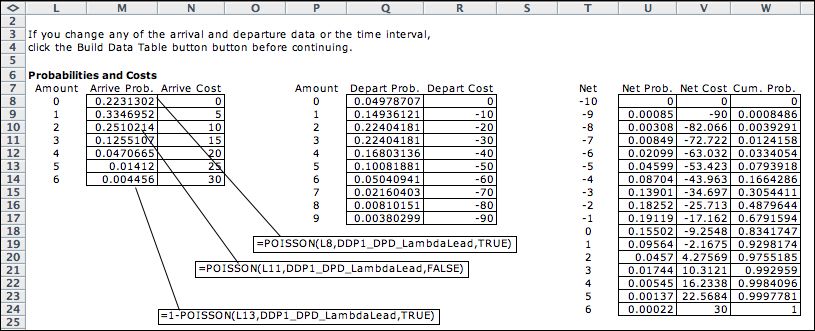
The range factor limits the range of the random variables
that are considered in the model. The Poisson random variable
is never negative, so 0 is a valid lower bound on the random
variable. The upper bound however is unlimited. To limit the
range we provide the range factors for demand and supply. For
the example they are both 3. We use this to truncate the distribution
by plus or minus (range factor)*(standard deviation). The standard
deviation for the Poisson is the square root of the mean. The
lower value is rounded down to the nearest integer, while the
upper bound is rounded up. The
limits for the example are (0 to 6) for supply and (0, 9) for
demand. For larger rates, the lower bound may be greater than
0. The probability columns are computed with the Excel Poisson function.
Clicking the Build Data Table button performs a convolution
to find the distribution of the net supply less the demand.
In the process we also calculate the net cost for each supply/demand
combination. The resultant distribution is shown in columns
T and U. The associated costs are in column V and the cumulative
probabilities are in column W. The cumulative distribution
is constructed only for deterministic models. The net distribution
is used in the for the DP model. |
|
Summary |
| |
The inventory data model has implementations
for all four problem types as described on the following pages. |
| |
|
|