 |
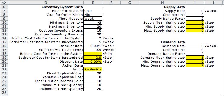
The data for the MDP
differs from the data for the DDP in that the MDP has no analysis
time. The MDP is an infinite time horizon model. The goal is
to minimize the expected cost of operation by choosing the
optimum action for each state. This is a stationary policy
that does not depend on time.

 |
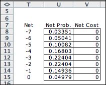
Since the rate of supply
is assumed to be 0 for this instance, the net supply minus
demand is entirely determined by the demand rate. The probabilities
are from the Poisson distribution. For the MDP demand is
not fixed but is governed by the Poisson distribution.
We assume that the distribution of demand does not change
over time. |
|
The Model |
|
The MDP model has three elements:
state, action, and event. These are shown in the figure
below. Cells colored yellow and outlined in red are formulas.
Most refer to a data item on the Data worksheet. When the data
worksheet is changed, the parameters of the model are automatically
adjusted by the formulas.
For the MDP, the state
is entirely defined by the inventory level (the stock). The
data allows backordered quantities so the range of the state
variable is [-5, 20]. Recall that the DDP requires two state
variables, time and stock level. The unit cost in F21 evaluates
the holding cost with a positive stock level and the negative
backorder cost when the stock is negative. The example state
value is (-2) so the unit cost is (-2.5). This results in a
state cost of 5.
The action element has two dimensions and is the same as with
the DDP. The first is the decision to
replenish or not, and the second is the lot size at replenishment.
A logical expression in J17 restricts feasible actions so that
the lot size must be 0 if the first decision is to
not replenish.
The event element is the demand on the system. The cost and
probability of the event are governed by the table computed
on the Data worksheet. |
|
| |
The Decision blocks shown below restrict
the set of state/action combinations that are feasible. When
decision blocks are included, feasible decisions must satisfy
one of the decision blocks. The first block sets the conditions
for a replenish decision. The state must be no more than
10 and the lot size must lie between 10 and 20. Data items define
these limits. They are used to reduce the set of decisions considered
in the optimization. The second block allows the no-replenish
decision for all states. |
|
| |
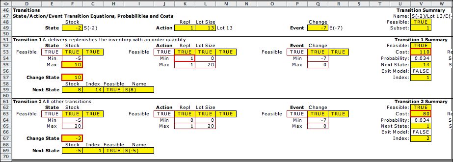
Transition blocks compute the transitions for
feasible decisions. The first block adds the lot size to the
state in the event of a replenishment. The second block changes
the stock level by the net demand. Both blocks evaluate as TRUE
for the example. In cases where more than one transition block
is TRUE, the block with the smallest index governs the transition.
For the example, it is transition block 1. |
 |
| |
To save space we do not show the inventory calculations
in the columns to the right of this display. The example has
a stock level of -2. When the demand is -7 as shown, the resultant
inventory would be -9 without replenishment. The inventory calculation
computes a shortage of 4 so the net change is -7+4= -3. This
result is shown in the Change State cell of block 2.
With a replenishment of 13 as indicated in K49 and K50, the inventory
changes by -7+4+13=10. This number is in the Change
State cell
of block 1. |
Lists |
| |
|
Clicking the List Elements button
initiates a program that enumerates all feasible states.
The states show possible values of the stock level. Recall
that the DDP model uses time as a state variable as
well as stock level and has over 800 states. Because the
MDP model has many fewer states it is easier to solve the
the DDP model. |
|
| |
|
The actions for the MDP are the
same as for the DDP. The first action is to hold the stock
without replenishment. The remaining actions allow replenishments
in lots of 10 through 20 units. |
|
| |
|
The eight events correspond to
the eight levels of demand (expressed as negative values).
The event describes the stochastic nature of this model. |
|
| |

...

|
The decisions are enumerated by
pairing all states with all actions. Those that satisfy one
of the decision blocks are listed in the Decision list.
There are 202 decisions compared with over 5000 for the DDP. |
|
| |

...

|
The DDP had one transition
for each decision. The MDP has eight transitions for
each decision, one for each value of the event variable.
These are enumerated by pairing each decision with each
event. There are 616 transitions.
The list at the left shows that several transition
entries may lead to the same next state. This is certainly
true for the state with the value -5. Every demand level
leads to a shortage, so a replenishment will add the
lot size to the stock level to find the next state.
|
|
| |
For the student interested only
in solving the MDP model for the inventory problem, it is unnecessary
to review these lists. For the student attempting some variation
of the model, the lists help to debug
a proposed model. |
Solution |
| |
Clicking the Transfer to DP Solver button
builds the solver model and transfers the list information to
the appropriate arrays in the solver model. The figure below
shows part of the solver model with the state information in
columns D through G. The decision and transition information
are in arrays to the right on the Solver worksheet. Columns
J and K show the optimum policy. The optimum reorder point
is a stock level of 2. Every stock level smaller than 2 also
requires a replenishment, The optimum lot size depends on the
state. With a stock of 2, the lot size is 13. For smaller values
of the state, the lot size increases.
The solution shown is the result of the Policy method
of solution. When the discount rate is 0, this method finds
the policy that minimizes average cost. The average cost per
step is in cell P11, or approximately 13.8. The probabilities
in column P are the steady-state probabilities when the optimum
policy is used. |
| |
|
Summary |
| |
The DDP finds the optimum solution for a simulated
demand. The replenishment decisions are computed for each step
in time. When the demand is a random variable, the MDP solution
does not find the optimum policy as a function of time. The
policy prescribes an optimum solution as a function of the
stock level. The policy is optimum for all time. The MDP problem
is considerably easier to solve than the DDP problem. |
| |
|


