|
|
|
|
| |
The Markov Chain
model requires three elements: states, events and transitions.
They are illustrated for the random walk problem. |
Random Walk Markov Chain |
| |
We use as an example
a random walk problem. The example here was constructed using
an early version of the DP Data add-in. The random
walk model now uses a somewhat simpler structure, but the one
shown is more concise. The random walk allows many alternative
assumptions that can easily be accommodated by the model structure.
In the example the random walk takes place on the
grid illustrated below. In the example the grid points range
from 0 to 3 in each of two directions. We call one direction
the N/S direction and the other the E/W direction. There is
a wall at 0 and another at 3 in both directions. This is a
Discrete Time Markov Chain (DTMC) model. The walker takes a
step in every time interval.
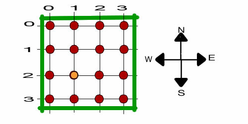
A walker wanders
around on the grid points randomly. Walls constrain
the walker. With the walker at some grid point, he can move
in any of four directions not constrained by a wall. The example
shows the walker as the yellow circle located at grid point
(1, 2). There is a fixed probability of traveling in any direction
and also a cost. When the walker tries to move in a direction
constrained by a wall, he simply does not move. There is no
cost associated with not moving. The table below, constructed
on the Model worksheet, contains the cost and probability
data as well as the transitions caused by the steps.
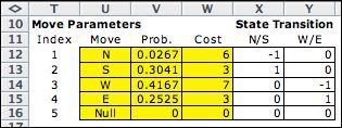
The model is shown below. The Markov
Chain model requires only the State and Event elements. In
this case the state variables describe the N/S coordinates
and W/E coordinates. The grid dimensions are reflected in the
minimum and maximum values for the state variables. The event
describes the Move,
with the moves 1, 2, 3, 4 and 5, representing N, S, E,
W, and Null respectively. Moves are governed by probabilities
and costs shown in cells L20 and L21. These cells contain formulas
that transfer values from the data table. |
|
| |
Transitions are defined
in the single transition block. The current state (2, 1) is in
the interior of the grid where all moves are possible. The
current event is to move South. The transition adds the Change
State vector (1, 0)
to the state vector to obtain the next state (3, 1). The new
state is shown in row 41. It is feasible and its index in the State
List is
14. All this is transferred to the summary portion of the model
that indicates that the state and transition are both feasible.
The model below shows state (3,
1) with the event move south. The Change
State vector (1, 0) designates a move
to south with the new state (4, 1). This move is not feasible.
The program knows this because the resultant state is not on
the state list (indicated by ##### as the index cell H41). This
feasibility test uses the list of states, so if the model
is modified by changing the state definition it is important
to click the List
States button
at the top of the page. |
| |
|
| |
The spinners (the double
arrows graphic) are used to increase and decrease a count index
by one. This is a useful tool for debugging a model. |
Building the Solver Model |
| |
The DP Models add-in
enumerates all feasible states and events and creates lists of
the elements of the problem. These are transferred to the DP Solver or Markov
Analysis add-in.
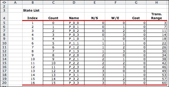
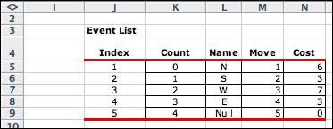
The lists are placed on a separate worksheet called RW_1_Lists.
The lists are shown below. There are 60 transitions. A Null event has been inserted whenever
the probability of the feasible events do not sum to 1. |
| |
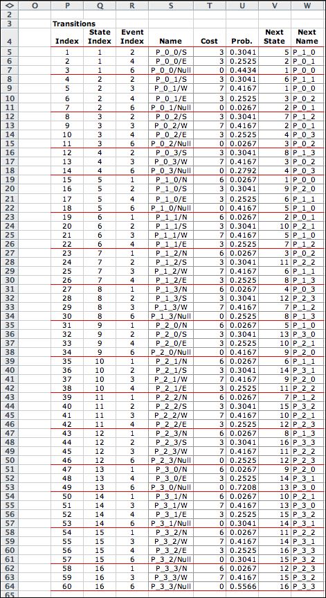
|
The DP Solver |
| |
Clicking the Transfer
to DP button, copies the lists to the DP Solver format.
There are three options for storing the transition structure.
Here we show the Probability/Cost Matrix structure.
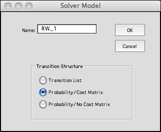
The top left of the DP Solver form is shown below. This is
the steady-state solution of the DTMC obtained using the Policy
method. The steady-state probabilities are in column
M. The State
Values in
column L are the steady-state NPW values for the chain. These
depend on the starting state. For the example, cell K14 gives
the NPW over an infinite time horizon when the system begins
at state (0, 0). This is the NW corner of the grid. |
| |
|
| |
The transition probabilities
in the matrix format are below. |
|
| |
The transition costs
are stored in a separate matrix. |
|
Transition Data Structure |
| |
An alternative structure
is to display the probability matrix, but
not the cost matrix. This reduces the storage required by replacing
the cost matrix with a column that holds the expected
transition cost.
A quite different option is the transition structure.
For this case the transition costs and probabilities are stored
in lists rather than matrices. Part of the transition structure
for the Markov Chain model is below. The table lists all feasible
state/event combinations. Transition costs are in column AD
and transition probabilities are in column AE. The index of
the next state resulting from the transition is in column AF.
The next state name is in AG. For larger state spaces, the
transition format uses many rows rather than many columns.
Since Excel allows many more rows than columns, larger problems
can be solved with this option. Also, most problems have a
relative few transitions per state. |
| |
|
Continuous Time Markov Chains |
| |
Markov Chain models can
also be constructed for continuous time (CTMC). The models are
very similar to the discrete time models except transition rates
are provided instead of transition probabilities. There is no
requirement that the rates must sum to a particular amount, so
Null events are not added to the transitions list. CTMC models
are not solved by the DP Solver add-in. The model page for a
CTMC includes a button that transfers the data to the Markov
Analysis add-in. |
| |
|


