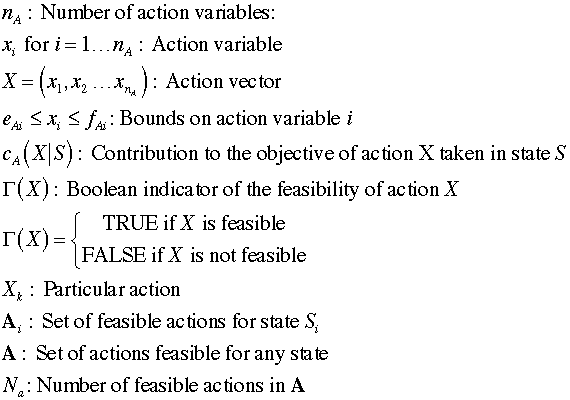
Actions are required for the deterministic dynamic programming models and the stochastic dynamic programming models (or the Markov decision problem). Every state, except an Exit state, admits one or more actions. Models with actions are optimization problems where the goal of the optimization is to minimize or maximize an objective function that depends on the sequence of actions.

In many ways the set of actions is similar to the set of states. The actions come from a finite set with each element of the set defined by a vector of integer variables. Actions always occur while the system is some state. The set of feasible actions and the objective contribution (or cost) of the action depend on the particular system state. For our models, however, we require that feasible actions be enumerable without recourse to the state. Thus we define an action element whose members depend only the lower and upper bounds of the action variables and perhaps additional logical conditions on the action variables.

Our models allow the objective contribution of the action to depend on the current state. The combination of a particular state and a particular action is called a decision. We provide Decision Blocks where each block represents a subset of state/action combinations. Each subset can have a specified objective contribution and an indication of feasibility. If a given decision (state/action combination) is not included in a defined subset it is not included in the analysis.

The Action Element

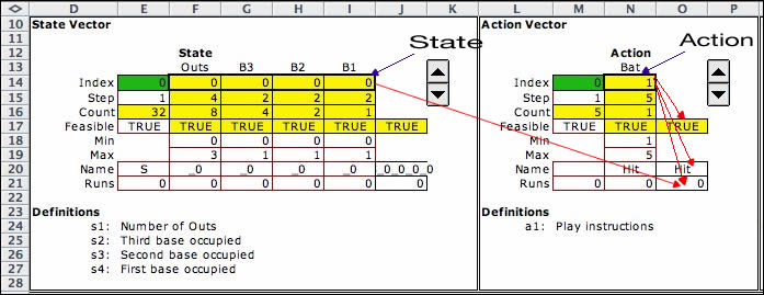
Actions are defined in the action element. It is located just to the right of the state element. The figure shows the state and action elements for the Baseball problem. The action element is identical in form to the state element. The baseball action has a single variable that holds the play instructions given by the coach. There are five possible instructions indicated by Min and Max bounds in rows 18 and 19. The current action is in cell N14, the integer 1 indicates the hit instruction. The remainder of the cells in this element play the same roles as they do for the state element. Row 21 describes the objective contribution for the action. The default is a linear function of the action variables. For the example, row 21 contains only zeroes. In general the values in row 21 can depend on both the state and the action.

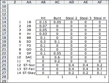
The set of available actions is found elsewhere on the worksheet in the data table shown below. The action titles are in the range (AB13:AF13). Cell N20 in the action element gets the action names using an INDEX function that points to this range. The rest of the data table gives information about the events of the situation.

Decision Subsets

The model allows decision subsets. The combination of a state and an action defines a decision. It is often convenient to use several decision subsets to indicate the feasibility or infeasibility of specific decisions. Also the objective function contribution may differ between subsets. Certain decisions may be identified as Exit decisions. An exit decision prescribes an immediate transition to the Finish state.

The baseball model uses five decision subsets designed to restrict the set of states that allow specific actions. They are pictured below. The subsets begin with a header region in rows 49 through 53 where the current state and current action are displayed. It holds the same state and action that appear in row 14 at the top of the page. The summary region in column X holds the name of the decision which is a concatenation of the state and action names. The value TRUE in S51 indicates that this decision is a member of one of the decision subsets. The value in X52 is the index of the subset that is feasible for this decision. The subsets must collectively include all feasible decisions. They need not be mutually exclusive. When a state falls in more than one subset, the one with the smallest index is indicated in X52. The current decision, S000/Hit is feasible and it is included in the fifth subset.

The subsets each occupy a range of the rows below the header. For example, Decision 1 defines the subset of decisions that allow the player to steal second base. For that decision to be feasible, the state must have first base occupied, B1=1, and second base empty, B2=0. The action "steal second base" is action 3. The logical condition and the bounds in columns E through I and M through N identify decisions that represent this situation. Since the current state has first base empty, B1=0, the conditions fail for this decision. Also the action index is 1, not 3. This result is reported in X55. X56 has the default value that is the action objective term. The formula in this cell can be changed to allow any function of the state and action. Cell X57 indicates that the decisions in this subset are not exit decisions. Cell X58 returns 9999 for an infeasible subset, and returns the index 1 when the subset is feasible.

The first three subsets identify decisions for stealing bases. Decision 4 allows the "Bunt" action only if there is at least one runner on base. This condition is described by a logical expression in E74:

=(G52+H52+I52)>0

This is true only when the sum of the base-state variables is greater than 0, or there is at least one runner on base.

The last decision subset allows the "hit" action for all states with two or fewer outs. The conditions for this subset are satisfied by the current decision and we say the decision is feasible.

It is not necessary to provide a decision subset for states with three outs since these have been previously been designated exit states. Exit states are assigned the decision "Null" since they require no decisions.

It is not required that decisions subsets be defined, but if one or more are used, then every feasible decision must be included in at least one decision subset. The change command allows the number of decision subsets to be increased or decreased, but will only allow additions if at least one is provided in the initial model setup. When no decision subsets are defined the set of decisions is determined by all possible combinations of feasible states and feasible actions.

Enumerating the Actions

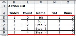
The DP Models add-in enumerates all actions defined by the action element. On the BB_Lists page column N holds the single state variable value. This happens to be the same as the index. Column O holds the objective function contribution for each action when the state vector is at its lower bound. In general if the decision contribution depends on both the state and action, column O plays no bearing on the model. It is useful for debugging when the action cost does not depend on the state.

.

Enumerating the Decisions

The enumeration process firsts enumerates all feasible states and then enumerates all feasible actions. Then each action is combined with each state to find the complete set of decisions. The MDP optimization will select the optimum decision for each state, so it is important the entire set of feasible decisions be enumerated.

Given a state and an action, the resultant decision is included in the model if the decision falls in one of the subsets. Otherwise it is not included. The decision list for the example is shown in part below. The example has 78 feasible decisions. At the top of the list we see that the state with all bases empty and no outs admits only the hit action. The state with no outs and first base occupied allows the hit, bunt and Steal 2 actions.

At the bottom of the list we see the states with three outs. Three outs signal the end of the inning. The state subsets define these as exit states. No decisions are enumerated for the exit states. Rather a single decision is indicated by the Null action.

When a state and action combination has no feasible decisions, the action "NA" is assigned to the state. The objective contribution for the NA action is a very large positive number for a minimization problem and a very large negative number for a maximization. When the optimum solution is determined using the DP Solver, states with no feasible actions are avoided if possible.

The next page addresses the model component called transition. These determine the changes in state that are engendered by the selection of a decision.

Other Examples

All optimization models include the action and decision components. This includes deterministic dynamic programming and MDP models. Some examples are below.

The Queue MDP has one action variable indicating whether to decrease the number of service channels, leave it the same, or increase the number of channels. The cost of the action is computed in cell M21 and is independent of the state.

The two decision blocks allow additions and subtractions to the number of service channels.

The Sequencing model describes the oil well sequencing problem. It involves six well locations and the decision problem is to find the optimum sequence to drill the wells. The action chooses the next well to drill or alternatively to quit before the sequence is complete.

The first decision block allows a selection of a well index (from 1 to 6). The states are not limited by the bounds in rows 40 and 41, but there is a formula in cell O39 that returns TRUE only if the corresponding cell in the state vector is -1 (not drilled). For the example the Drill 3 action is feasible because the value of s3 is -1. This means that site 3 is not yet drilled. The second decision set is an illustration of an exit decision. If the action is to quit (action 7), the decision will go directly to the Final state.