|
|
 |
Dynamic
Programming Models |
 |
-
Models: Events/Transitions |
|
|
|
|
| |
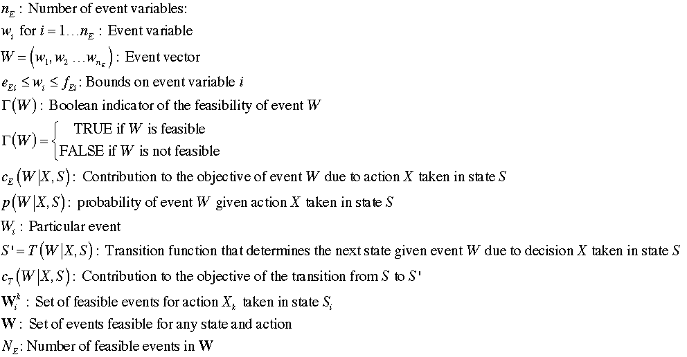
Events describe the stochastic
features of the model and the transitions from one state to
another. Events are necessary for Markov Chain and MDP models,
but not deterministic DP. Transitions are also included for
the deterministic DP models, but they depend only on states
and actions.
In many ways the set of events is similar to the sets of
states and actions. The events come from a finite set with
each element of the set defined by a vector of integer variables.
Events always occur while the system is under
control of some decision. Recall that a decision is the combination
of a particular state and a particular action.
The set of feasible events, the objective contribution, and
the probability of occurrence of the event depend on the decision.
For our models we require that all possible events
be enumerable without recourse to the decision. Thus we define
an event set whose members depend only the lower and upper
bounds of the event variables and perhaps additional logical
conditions on the event variables.

Our models allow the objective contribution and
probability of the event to depend on the current decision.
The combination of a particular decision and a particular event
results in a transition.
The transition function is the functional relationship that
determines the values of the state variables of the next state.
The transition moves the system from the current state to some next
state,
perhaps the same as the current state. We provide Transition Blocks where
each block represents a subset of decision/event combinations.
Each subset can have a specified objective contribution, probability,
transition function and an indication of feasibility. If a
given transition (decision/event or state/action/event combination)
is not included in a defined subset it is not included in the
analysis. All models have at least one transition block. |
The Event Element |
| |
Events
are defined in
the event element.
It is located just to the right of the action element.
When actions are not defined, as with Markov Chain models,
the event element is next to the state element. The
figure shows the state, action and event elements for the Baseball problem.
The event element is identical in form to the other two elements.
The baseball event has a single event variable that
describes the play outcomes.
There are fourteen possible results indicated by Min and
Max bounds in rows 18 and 19 of column S. The current
event is in cell S14, the integer 1 indicates the 1B result,
a one base hit. Row 20 contains the event contribution to the
objective function. This information is more readily defined
in the transition blocks so we enter 0 here. Row 21 holds information
for the probability of the event. The red arrows below indicate
that both the state and action, as well as the event, may affect
the objective contribution and probability of the event. The
name and feasibility only depend on the event variables.
The default formula for the event objective contribution
is a linear function of the event variables. The default formula
for the event probability is the product of the contents of
cells R21 and S21, but here a table INDEX function places the
appropriate value in S21. The formula in
cell S21 is
=INDEX(AB14:AF27,BB_DPM_Event,BB_DPM_Action)
Cell T21 sums the contents of R21 and S21, so
it is the same as S21. |
|
| |
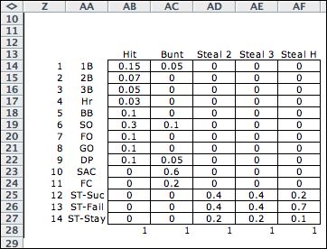
The event
titles are in the second column (AA) of the data table below.
The probabilities depend on both the action and event. For
the current action of Hit, the event of a one-base
hit has the probability of 0.15. The possible events for each
action are mutually exclusive and their probabilities sum
to 1.

|
Transition Blocks |
| |
The decision/event
combination results in a transition. It is necessary to provide
a transition function that determines the next state. Transition
functions are provided by the transition subsets. I call the
part of the worksheet that defines the transition subset
a transition block. Because of the complexity of baseball,
there is no simple function that is valid for all decision/event
combinations. The simplified game considered by our model requires
26 transition blocks. Several of them are shown below. This
part of the worksheet starts at row 90 with a repetition of
the current state, action and event. For this example the state
indicates that there are no outs and the bases are empty. The
coach has called for a hit (action 1) and the result is a one-base
hit (event 1). Column X summarizes the results of the results
of the blocks that follow. We see the name of the transition
in X92, the TRUE in X93 indicates that the transition is feasible,
the 1 in X94 indicates that the objective contribution, probability
and transition function of block 1 holds information
concerning this transition.
All transition blocks contain the bounds and logical conditions
that determine whether the block is appropriate for the
current decision/event combination. Block 1 is feasible if
the number of outs is two or less, with any pattern of
bases full or empty, the action is 1 or 2 (hit or bunt) and
the event is 1 (one-base hit). Block 1 is feasible for the
example. Other blocks might also be feasible, but only the
top feasible block is reported.
A one-base hit advances each runner to the next base and places
the batter at first base. If third base is occupied before
the hit, that runner scores a run. This is described in the Change
State region in row 96. The change state vector
is added to the current state vector to find the next
state. There is
no change in the Outs value.
The formulas in the Change
State cells that represent bases, move the runner from
one base to the next. The formula in the Runs column evaluates
to 1 if the third base is occupied. The next state is reported
in row 98 as (0,0,0,1). An Excel function looks up the next
state to see if it is on the state list. If so, the index of
the state is reported in J98. Cell K98 returns TRUE to indicate
that the new state is feasible and L98 reports the name of
the next state.
| Cell |
Outs |
B3 |
B2 |
B1 |
Runs |
| State |
0 |
0 |
0 |
0 |
|
| Change State |
0 |
=-G$88+H$88=0 |
=-H$88+I$88=0 |
=-I$88+1=1 |
=G$88=0 |
| Next State |
0 |
0 |
0 |
1 |
0 |
The report is summarized in column X starting in row 91. The
transition block is feasible (X91) if the feasibility conditions
for the block are satisfied and the next state is feasible
or designated as an exit transition. The contribution in runs
is in X92. The probability of the transition is 0.15 (cell
X93). Generally this cell is a repeat of the event probability
unless a different formula is placed in this cell. The
index of the next state is 2 (X94). an exit transition can
be specified by placing TRUE in X95. This causes a transition
to the final
state regardless
of the feasibility of the next state. Cell X96 reports the
index of the transition block as 1. If the block is not feasible,
this cell will report 9999. The value in X96 is used by the
expression in cell X88 to determine the transition subset appropriate
for a specific decision/event combination. |
|
| |
The selection above
shows some of the easier transition formulas. Some plays are
difficult to describe generally, especially the double play
and fielder's choice results. The interested reader can see
the transitions used by this author in the baseball
excel file. More discussion can be found in the baseball
article in the DP Examples section. |
Enumerating the Events |
| |
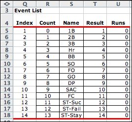
The DP Models add-in
enumerates all events defined by the event element.
. |
Enumerating the Transitions |
| |
The enumeration process
firsts enumerates all feasible states, all feasible
actions and all feasible decisions. Feasible states are combined
with feasible actions to obtain the list of feasible decisions.
Then the feasible decisions are combined with feasible events
to find the collection of all transitions from all decisions.
The list of transitions is placed on the BB_Lists
worksheet. We show parts of both the decision and transition
lists for the baseball model. Each decision has several transitions.
For example the (0,0,0,0) state with action 1 (Hit with the
bases empty and no outs) has nine transitions. Only transitions
with nonzero probabilities are included. Some transitions result
in runs scored and others do not. Each transition has a probability
and the index of the next state. More than one transition may
result in the same next state. Some transitions may return
to the same state. There are 402 transitions for our baseball
model. |
| |
|
| |
At the bottom of the
list we see the states with three outs. Three outs signal the
end of the inning and have been defined as exit states. No decisions
or transitions are enumerated for the exit states. Rather,
a single decision is indicated by the Null event. Each of the
Null decisions is followed by a Null transition as shown in
the last few transitions. All go to the final state (state
33). The final state is a recurrent state. Once the system
arrives in the final state the inning is over.
All the events for a decision must be mutually exclusive.
If the probabilities of all the feasible transitions for a
given decision do not sum to 1, an additional transition is
provided that represents the null event. The null event returns
the system to the same state with 0 contribution to the objective.
If there are no feasible events for a decision, the transition
returns to the same state with probability 1 and the state
is said to be recurrent for this decision. |
Why the Model? |
| |
All this effort is
to construct the five lists: state, action, event, decision
and transition. These are necessary to describe the problem
to the DP Solver. Even though this
is a relatively simple model of the baseball inning, it is complex
enough to provide a challenge in understanding the underlying
situation and formulating it through the mechanics of our DP
Models add-in. This would be very difficult without a structured
approach to modeling the situation in abstract terms and allowing
the computer to generate the detailed features of the abstraction.
The numbers of states, actions and events for the baseball
problem is small relative to most real-world problems. It is
the product of these three numbers that determines the complexity
of the modeling and solving processes. Although this quantity
grows linearly with the parameters rather than exponentially,
the numbers of transitions easily grows beyond the capacity
for imagination. The number of transitions does grow exponentially
with the number of state variables, action variables and event
variables. Only
the abstraction provided by the modeling tool makes even small
problems possible. |
Other Examples |
| |
All models involving
risk include the event component. This
includes Markov Chains and MDP models. Some examples
are below. |
| |
The Doors problem
is a random walk model with a single event variable representing
the event of moving in one of the four direction. State P_0_0
and P_3_3 are absorbing states. The actions involve blocking
movement in one of the four directions. When not blocked the
transition probabilities are 1/4. When one direction is blocked,
the transition probabilities are increased to 1/3 in the non-blocked
directions, leaving the blocked direction with zero probability.
The probabilities and transitions are described by columns
AG through AI of the transition list.
|
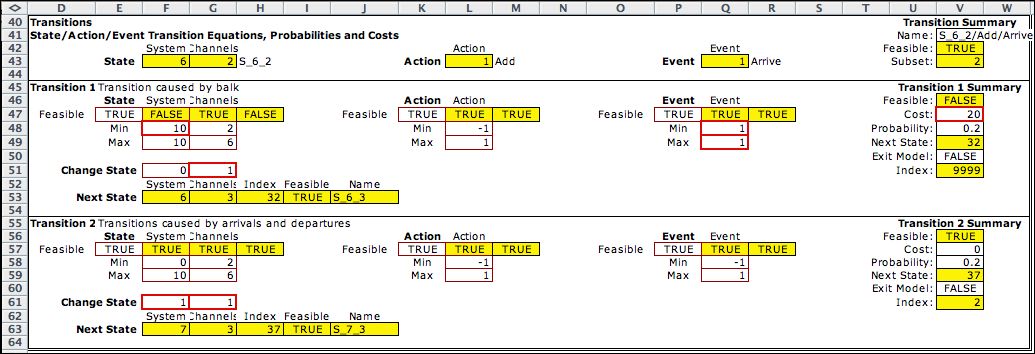
The Queue MDP
has one event variable indicating whether an arrival, departure
or neither has occurred.
The two transition blocks allow either a balk or the acceptance
of an arrival or a departure. The balk event occurs only when
the system is full. The departure event when the system
is empty is not explicitly rejected. It is not included in
the transition list because the list does not accept transitions
that do not lead to a feasible state. The example shows a transition
when an arrival occurs and the action adds a service channel
to the system. The system changes from state (6,2) to (7,3). 
|
| |
The Sequencing model
describes the oil well sequencing problem.The event variable
has only two values indicating the success or failure of drilling
a well. A few of the many transitions are shown in the table.
|
|
| |
|
|


