|
|
 |
Dynamic
Programming Models |
 |
-
Models: States/State Subsets |
|
|
|
|
| |
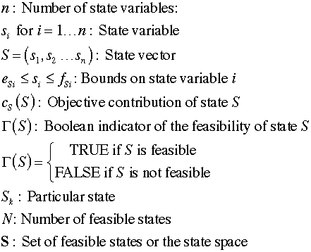
The states of the
system are described by the following notation. In our models
there is a finite number of states and each state is represented
by a vector of n elements called state variables.
Each state variable is discrete and has a finite
number of possibilities. In all our examples the state variables
are integer.
|
The State Element |
| |
The model
is described on a range of the models worksheet,
called the state element.
It is illustrated for a particular case for the states of the Baseball problem.
Each state variable has a column of cells in the state element.
For the example there are four state variables. The first state
variable in column F indicates the number of outs in the inning.
The remaining three state variables, B1, B2 and B3, indicate
the status of the bases where each base has a runner or not.
In the example, third base is in column G, second in column
H and first base in column I. Lower and upper bounds on the
state variables are in rows 18 and 19 respectively. The interval
between one state variable value and the next is the Step size
in cell E15. A step of 1 means that each state variable takes
on consecutive integer values between the lower and upper bounds.
The bases are listed in the order shown because it more convenient
for reviewing the lists produced by the enumeration. It is
the same order used by Howard who originally proposed the problem.
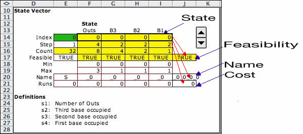
The value of the state variables are in the range
(F14:I14). The figure shows the state (0,0,0,0). In terms of
baseball, this is the situation with no outs and the bases
empty. Rows 15 and 16 hold formulas that are used by the enumeration
process. Cell E14 holds an integer value that corresponds
to a particular state. The value 0 indicates (0,0,0,0). The
value 31 indicates (3,1,1,1). The number of state vectors is
equal to the number in E16, 32 in this case. The complete set
of states is enumerated by allowing the number in E14 to range
from 0 to 31. The spinner control in column K changes the number
in E14 by integer amounts. This is useful for manually debugging
the model.
The conditions for a feasible state are in row
17. Cells in the range (F17:I17) hold logical expressions that
return TRUE if the state variable is within its lower and upper
bounds. Cell E17 has a default value of TRUE, but a user defined
logical expression can be inserted in cell E17 that imposes
additional conditions on feasibility. Cell J17 indicates the
feasibility of the current state. It returns TRUE if all cells
in the range (E17:I17) are TRUE. Otherwise it returns FALSE
and the state is not feasible.
Rows 18 and 19 hold lower and upper bounds on
the state variables. All the examples use integer values of
the bounds.
Row 20 holds string formulas and constants that
define the name assigned to the states. Cell J20 is the specific
name for the state. In the figure it is partially hidden because
the width for column J is too small, but the value is S_0_0_0_0.
Cells F20 through I20 hold formulas that combine the underline
symbol with the state variable value. Cell J20 concatenates
the values in the range (E20:I20). Names are useful for interpreting
and debugging the model. In later versions of the DP Models
add-in, the name uses commas rather than the underline symbol
and begins and ends the name with parentheses. The example
state has the name (0,0,0,0).
Cell J21 holds the state contribution to the
objective function. Initially the cell holds a formula that
is a linear expression of the cell values plus a term computed
in cell E21. The coefficients of the linear expression
are in the range (F21:I21). The default values are
0. Cell E21 also is initially 0. Cell J21 is
the sumproduct of the ranges (F20:I20) and (F14:I14) plus
the value in E21. The contents of (E21:I21) and the formula
in J21 can be manipulated by the user to represent any
single valued function of the state variables. Dynamic programming
places no restrictions on the form of the objective function
components except that they be computable, well defined and
single valued. This flexibility is one the strengths of the
dynamic programming model.
For the baseball problem, the objective is to
maximize the number of runs scored in the inning. Thus the
objective row takes the name Runs rather than Cost.
We often use the term cost to indicate the general objective
function terms, but most problems have a specific measure that
is more relevant.
The red arrows in the figure indicate functional
dependence. The feasibility, name and cost calculated in column
J all depend functionally on the state vector. Entries in the
other columns are provided to accept terms
that are combined, usually by addition, to yield the result
in column J. The values in column J and the state specified
in row 14 are used in other parts of the worksheet. |
State Subsets |
| |
For many situations
it is difficult to completely define the features of the states
with the state element alone. Some states may be infeasible
and the objective value may be a complicated function of the
state variables that differs between different sets of states.
To simplify modeling, we provide the option of state
subsets. State
subsets allow modifications to the feasibility and objective
function values computed in the state element. They also allow
states to be identified as exit states.
Models do not require state subset definitions, but if one
or more are created, the collection of subsets must include
all feasible states. States left out by the subset definitions
are judged infeasible and not included
in the state set. The subsets are not required to be mutually
exclusive. If a state is included in more than one subset,
the one with the smallest index (or nearest the top
of the worksheet) is used.
The baseball
model defines the two state subsets shown below. The subsets
begin with a repetition of the current state in the range (F33:I33).
The state vector is transferred directly from row 14 of the
state element. It is repeated in row 33 for easy reference.
When formulas in the state subsets refer to the state, they
should reference the values in row 33 rather than row 14. Information
in column X of rows 32 through 34 provide summary information
regarding the subsets. When X33 is TRUE, the current state
falls within one of the subsets. When it is FALSE no subsets
hold the current state and it is not included in the model.
For a feasible state, the values in both cell J17 and X33 are
TRUE. |
|
| |
The subsets are defined
by bounds on the state variables and a logical condition that
must be TRUE for states to be included in the subset. For example,
the first state subset represents all states
that have three outs, or the value 3 as the first state variable.
The lower and upper bounds in cells F33 and F34 are both 3.
Any state that does not fall within the bounds is not a member
of this subset. The other state variable bounds are 0 and 1,
the same bounds as in the state element. So these new bounds
are not restrictive. Cell E38 allows a logical expression that
must be TRUE for all elements of the subset. The default value
is the constant TRUE, but the cell can be changed to represent
other logical conditions. Cell J37 is TRUE if all cells in
the range (E38:I38) are TRUE. The state (0,0,0,0) does not
satisfy the logical conditions for the first subset so this
state is not in the subset.
Features of the subset are expressed in column X. X35 returns
the same value as J37, so it indicates whether the current
state is in the subset. Cell X36 has a formula that points
to the objective value formula in the state element, cell J21.
The formula in X38 can be changed to represent the objective
value contribution specific to the subset. When a state falls
within the subset, the subset objective value takes precedence.
Cell X37 holds a logical constant that when TRUE indicates
an exit state. An Exit state completes the sequence of states
and there are no actions or transitions to be taken from that
state.
Cell X38 returns the subset index when the current state is
in the subset. Otherwise it returns 9999.
Here it is 9999 because the current state does not have three
outs. Cell X34 is determined by the minimum of
the subset indices. If it is less than 9999, cell X34 indicates
the subset with the smallest index. Cell X33 returns TRUE when
X34 is less than 9999.
The second subset in the example represents all states with
2 or fewer outs. This is expressed by the bounds 0 and 2 in
cells F45 and F46. The current state (0,0,0,0) does meet the
logical requirements of the second subset, so cell X43 returns
TRUE. State (0,0,0,0) is in the second subset.
The state subsets are shown below for (3,1,1,1). This state
is in the first subset, so it is identified as an Exit state.
The objective contribution for an exit state is the value in
the objective cell of the associated subset. For the example,
the contribution to the objective for states with three outs
is in cell X38. That value is zero. Exit states can play a
variety of roles in a model. The exit state will indicate an
infeasible state if the objective contribution is set to a
very high value for a minimization problem or a very low value
for a maximization problem. |
| |
|
Enumerating the States |
| |
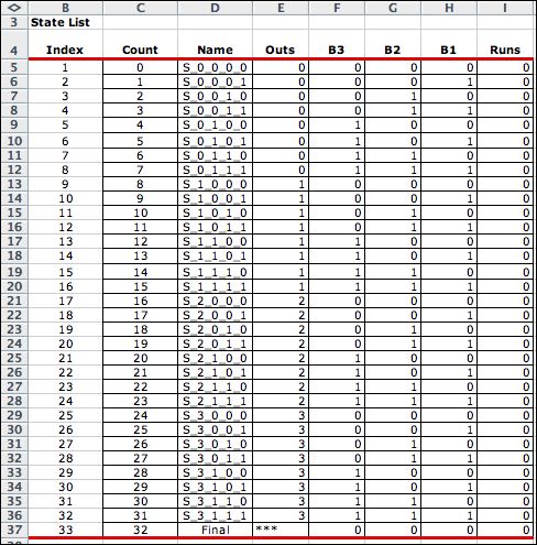
The DP Models add-in
enumerates all states that satisfy the bounds in the state element
and creates the list of all feasible states. The list for the
baseball problem is below. Thirty two states are identified by
the enumeration. For models that have exit states, one additional
state called the Final state
is added to the model. For the first 32 states, each row designates
the index, the count value, name, state variables and objective
contribution for a single state. The state indices in column
B are used to refer to the state in other parts of the model.
The Final state
has the greatest index and a non-numerical value for the first
state variable. For all states except the Final state, the count
value is the unique integer that when placed in cell E14 determines
the current state on the model worksheet. The states are sorted
according to the state variable values. |
| |
|
Other Examples |
| |
Each model has a state definition
that is appropriate to the situation. There are a number of examples
within this Dynamic Programming section. Some are shown
below. |
| |
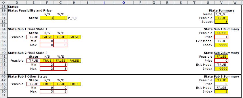
The Doors problem
has two state variables representing the coordinate points
on a grid. The problem is a random walk with trapping states.
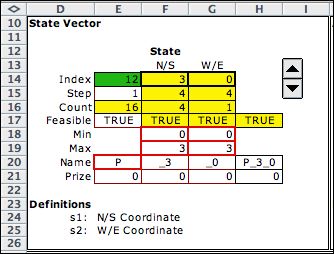
The state subsets identify two exit states.
The third state subset includes all states including those
identified by the first two subsets. When a state falls within
one of the two subsets, the results of the highest (smallest
index) are used. Note that exit state (0,0) wins a prize of
1, while exit state (3,3) wins no prize. The optimization maximizes
the total prize for the random walk so it encourages actions
that lead to state (0,0).
|
| |
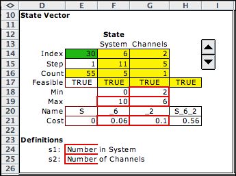
The Queue MDP
has two state variables, the first represents the number
of customers in the queuing system and the second represents
the number of service channels. No state subsets are required.
The model allows the number of servers to vary between 2 and
6. The state cost reflects a cost of 0.06 for each customer
waiting or in service and a cost of 0.1 for each server. The
time interval is minutes, so both coefficients represent the
cost per minute. The objective contribution is a linear function
of the state variables and the coefficients in row 21.
|
| |
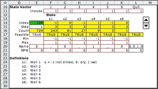
The Sequencing model
describes the oil well sequencing problem. It has states for
each well location. The state variables indicate whether the
well has been not drilled, drilled and found dry, or drilled
and found wet.
|
| |
|
|


