|
|
 |
Dynamic
Programming Models |
 |
|
|
|
| |
|
The DP Models add-in provides a structure to abstractly
define several kinds of models. These are listed in the dialog
below and illustrated by the pages in this section. |
|
| |
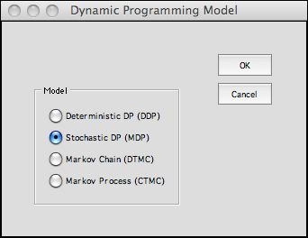 |
The first step is to choose the kind of model.
Four model types are allowed. The most general is the Markov
Decision Process (MDP) or equivalently the Stochastic
Dynamic Programming model.
We illustrate the types in this section.
The best
instruction is to review illustrations of the models. Some
of these are in the Examples section
of the DP Collection. Others are in the DP
Data pages. |
|
| |
The DP Models
add-in does require some skill at using Excel formulas, but
much of the model generation is performed at the click of a
button. For the beginner it is best to work with the DP
Data add-in. This DP Data add-in calls the DP Models
add-in to build model forms and then fills the forms with the
appropriate formulas and constants. With only a few changes,
the models provided can be modified to represent significant
problems that arise in practice.
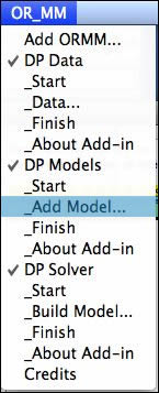
The Start command places all buttons required by
the DP Models add-in on the worksheet. This may be
necessary when a workbook created by one computer is opened
on another computer.
The Finish command
removes all the buttons. This makes
it simpler to open a data file on a different computer without
generating a link error message. It is better to remove the
buttons before saving. Use the Finish command to accomplish
this. When a workbook is subsequently opened, the Start command
makes the worksheets functional. The example files for this
add-in have been saved with the buttons removed.
We show the menu with the DP Solver add-in installed.
It must be installed to analyze DP models. The DP Models add-in
also makes models that can be analyzed by the Markov Analysis
add-in. |
Elements |
| |
The dynamic programming
model is comprised of several elements. The elements
for the MDP are the states, actions, events, decisions and
transitions as illustrated in the picture.
The red circles are the states. At each state the decision
maker must choose one from a given set of actions. The actions
are indicated by the red lines connecting to the black circles.
We call the combination of state and action a decision.
The figure shows two decisions for state 1. At each decision
there is a set of events that may occur. Each event has a known
probability and the sum of the event probabilities for a decision
is equal to 1. Each event results in a transition from the
decision node to a state node as indicated by the black lines.
The picture shows three events for decision 1 and two events
for decision 2. The complete model must define all feasible
states, all feasible actions, all feasible events, all feasible
decisions for each state, and all possible transitions from
each decision. Each state must have at least one
action, and each decision must have at least one transition.
In the following discussion we add one element to the five
already defined called the state subset.

The model describes a sequential process that
proceeds in steps. Beginning in some state the decision maker
chooses an action. Given the state and action an event occurs
according to a discrete probability distribution. The event
moves the system to a new state. The process continues to the
next step where a second action is chosen and an event occurs
leading to third state. The process continues in this sequential
manner. For some problems a final state is identified. The
process ends at when it reaches the final state. For other
problems the process never ends but continues wandering through
the states for an infinite number of steps.
The model must provide the set of actions available
for each state, the set of events that can occur for each
state/action combination (decision) and the probability
of each event. The MDP problem has an objective that is to
be minimized or maximized by the actions chosen. The model
must identify the contributions of states, decisions and transitions
to the objective at each step.
Because of the wide range of problems that can
be described by a model of this kind, it is difficult to provide
a model structure that is general. Linear and integer linear
programming models are simple in concept because of the restriction
to linearity for the objective function and constraints. Many
excellent modeling tools are available for LP and IP, and they
are useful for very large practical problems. This section
describes a general model form constructed on an Excel workbook
that seems to be useful for a variety of problems that are
related to DP. It is too early to tell if the structure is
sufficient for all problems that involve states, actions and
events, but it has been used for several problems that have
appeared in the literature. Some are described in this dynamic
programming section. |
Different Problems |
| |
The table below shows
the six elements of the DP model. The X values indicate that
the element is required, and "Optional" indicates
that the element may be used, but is not required.
|
States |
Actions |
Events |
State
Subsets |
Decisions |
Transitions |
| Markov Chain |
X |
|
X |
Optional |
|
X |
| Deterministic DP |
X |
X |
|
Optional |
Optional |
X |
Stochastic DP
or Markov Decision Process |
X |
X |
X |
Optional |
Optional |
X |
States and transitions are required for every model type.
Actions and decisions are added for optimization problems.
Events are added for problems involving probabilities. The
optional elements are useful for restricting combinations that
are infeasible. For example the State Subsets element
is used to identify subsets of states that have different characteristics.
Most deterministic DP models start at some Initial state
and finish at one or more Final states. The State
Subset element is used to define the states where the
process terminates.
The Decisions element deals with combinations of
states and actions. Although these are defined independently
in the State and Action elements, for many
problems it is important to identify state and action combinations
that are infeasible or have different objective function formulas.
The combination of a state and an action is called a decision.
The Transition element deals with combinations of
decisions and events for optimization problems that involve
probabilities. This is the MDP problem or stochastic dynamic
programming. For Markov chain problems, the transitions depend
on combination of states and events. For deterministic dynamic
programming the transitions depend on combinations of states
and actions. |
Model Element Dialog |
| |
In the following pages
we use the Baseball problem
for illustration. This problem concerns a single inning of
the baseball game. The goal is to maximize the number of runs
scored in the inning. As we will see in the pages to follow,
the inning begins with no outs and no one on base and ends
when the third out occurs. The elements of the problem are
entered in the following dialog. There must be at least one
state variable, one action variable and one event variable.
These numbers can't be changed after the model is constructed.
State, decision and transition blocks divide the associated
elements into subsets for easier modeling. Their numbers are
entered here. If more than one is initially specified, the
change button will allow addition or deletion of blocks. If
the initial value is 0, the number of blocks cannot be changed.
The economic measure, time unit, discount rates will
be reflected on the worksheet. When the maximize objective button
is checked, the objective function will be maximized, otherwise
it will be minimized. When the computation columns entry is
nonzero, extra columns are identified to the right of the model
form. These are handy for numerical computations related to
the model elements. They are used in the Inventory example.

Near the top of the dialog is the Include Stage State button.
When this button is checked an additional state variable is
included to designate the stages of the model. If the button
were clicked on the BB dialog, there would be five state variables
rather than the four specified, and the stage state variable
would be the first state variable on the model worksheet. Although
stages are important in many textbook descriptions of dynamic
programming, they are only necessary for finite horizon models
where the stages differ in some structural feature. All our
examples, except the resource examples and the deterministic
inventory model, are defined without stages. The extra dimension
associated with the stages markedly increases the size of the
DP model and, if possible, the stage option should not included.
The Include Step Size button determines the step
size between consecutive values of the state variables, action
variables and event variables. The default value, the integer
1, is sufficient for most problems and is the assumed value
when this button is not checked. When the button is clicked
the element forms are amended to include a step size. Steps
may be positive value. Take care when using steps that all
elements, states, actions and events, have comparable step
sizes.
The dialog is somewhat different for the Markov Chain and deterministic
dynamic programming models. The following pages first
describe the elements and then show how the elements are
used in the three classes of problems. |
Parameters and Buttons |
| |
Clicking the OK on
the dialog calls subroutines in the DP Models add-in to create
a worksheet for the model. The top-left corner of a model page
is shown below. Parameters of the model are in columns A and
B. The yellow range in column B should not be changed because
it holds structural information concerning the model. The
white cells can be set to show the economic measure, time measure,
discount rate and goal.
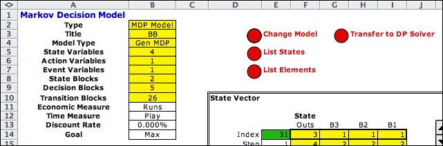
The red buttons to the right call subroutines to perform various
functions. The three buttons in column
D are common to all the model types. The buttons in column G
differ by model type.
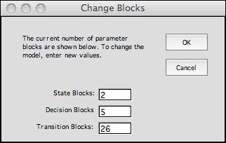
The Change Model button presents a dialog through which
the number of blocks for a model can changed. The dialog below
is presented with the current numbers of blocks of the three
types. The number of a particular type cannot be changed if it
is initially 0.
The List States button is used during
the debugging process. This button creates a list of states on
a separate sheet of the workbook. The transition blocks refer
to this list to determine if a transition is feasible. Whenever
the state definition is changed on the model worksheet it is
good to click the List States button.
The List Elements button lists all the
elements of the model. Again, these lists help to debug a model.
The designer should study these lists to make sure that they
reflect the situation being modeled.
The Transfer to DP Solver lists all the
elements of the problem, creates a worksheet for the data for
the DP Solver, and transfers the list contents to the solver
worksheet. |
| |
|
|