|
|
 |
Dynamic
Programming Models |
 |
-
Deterministic Dynamic Programming |
|
|
|
|
| |
We use a problem from
the Models section
of this site to illustrate the use of the DP Models add-in for
a Deterministic Dynamic Programming problem. Go to the Investment
Problem page to see a more complete description.
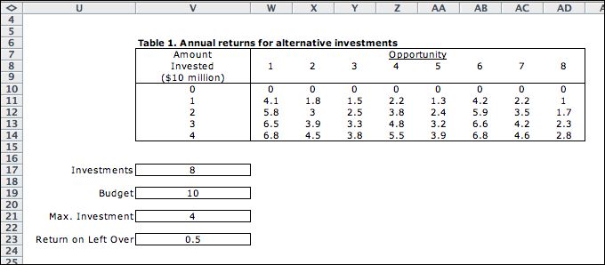
A portfolio manager with a fixed budget of $100 million
is considering the eight investment opportunities shown
in Table 1. The manager must choose an investment level
for each alternative ranging from $0 to $40 million. Although
an acceptable investment may assume any value within the
range, we discretize the permissible allocations to intervals
of $10 million to facilitate the modeling. This restriction
is important to what follows. For convenience we define
a unit of investment to be $10 million. In these terms,
the budget is 10 and the amounts to invest are the integers
in the range from 0 to 4.
Table
1. Returns from Investment Opportunities |
Amount |
Opportunity |
Invested
($10 million) |
1 |
2 |
3 |
4 |
5 |
6 |
7 |
8 |
0 |
0 |
0 |
0 |
0 |
0 |
0 |
0 |
0 |
1 |
4.1 |
1.8 |
1.5 |
2.2 |
1.3 |
4.2 |
2.2 |
1.0 |
2 |
5.8 |
3.0 |
2.5 |
3.8 |
2.4 |
5.9 |
3.5 |
1.7 |
3 |
6.5 |
3.9 |
3.3 |
4.8 |
3.2 |
6.6 |
4.2 |
2.3 |
4 |
6.8 |
4.5 |
3.8 |
5.5 |
3.9 |
6.8 |
4.6 |
2.8 |
Table 1 provides the net annual returns from the investment
opportunities expressed in millions of dollars. A ninth
opportunity, not shown in the table, is available for
funds left over from the first eight investments. The
return is 5% per year for the amount invested, or equivalently,
$0.5 million for each $10 million invested. The manager's
goal is to maximize the total annual return without exceeding
the budget. |
|
Creating the Model |
| |
This problem is not
addressed by the DP Data add-in, so we create a problem
by choosing the Add Model menu item from the DP
Models add-in. Select the Deterministic DP option
and click OK. A second dialog asks for the parameters of
the model.
A deterministic DP has states and actions, but no events.
Click OK to initiate the model building process. The figure
below shows the top part of the form. The form is shown after
it has been modified for the investment problem. The goal is
to maximize the total return so we use a discount rate of 0%.

Data required by the analysis is placed to the right of the
model. The data is linked to the model using Excel formulas.
If the data changes, the model automatically adjusts.

|
Filling the Model Form |
| |
The figure below shows
the model form after it has been filled in. The yellow fields
hold formulas that should not modified. The green fields hold
computer generated results, but they can modified by the user
when debugging the model. The white fields hold formulas or numbers
provided by the user.
There are two state variables, the investment opportunity
and the amount of the resource already spent. The current state
(1, 0) is in F14 and G14. This is the initial state where
the first opportunity is being considered and none of the budget
has been spent. Rows 18 and 19 hold the lower and upper bounds
on the state variables. When constructing the Solver model,
the computer will consider all states within these ranges.
The actions ranges from 0 through 4 indicating the amount
to invest. The Return in L21 holds a pointer
to the data table. The return is a function of both state (the
opportunity) and the action (the investment). The action shown
invests 3 in opportunity 1 for a return of 6.5.
The model has a single transition block, starting in row 52,
that governs all transitions. The most interesting aspect of
this is the Change State vector. The number 1 is placed
in cell F58 because a transition always moves to the next opportunity.
Cell G58 holds the change in the budget spent with the current
action. In this case, it is the value of the action
given in cell L50. The figure shows that
the action 3 taken while in state (1, 0) leads to state (2, 3). |
|
| |
Notice there are two
state subsets starting at row 28. The first subset starting in
row 34 defines the exit states of the model. It is always necessary
to define these because the system must terminate. The
bounds on this subset specify that the final states all have
the first state variable equal to 9. The second subset, places
no additional restrictions on the state variables, so this
subset represents all states except those defined by the first
subset.
The figure below shows a final state (9, 5). Cell Q36 has a
formula to evaluate the final states. When 5 remains unspent from
the budget, the return is 2.5. Both state subsets are TRUE for
this example. The program always selects the top subset when
more than one condition is satisfied. |
| |
|
| |
The transition formula
holds for all feasible actions taken from all feasible states.
Some actions taken from feasible states do not reach a feasible
state, however. For example, the state is (4, 9) indicates opportunity
4 with an amount spent of 9. An investment of 3 results in a
transition to (5, 12). The transition is infeasible because (5,
12) is not a feasible state. Only transitions to feasible states
(those in the state list) are enumerated. |
| |
|
Enumerating the Elements |
| |
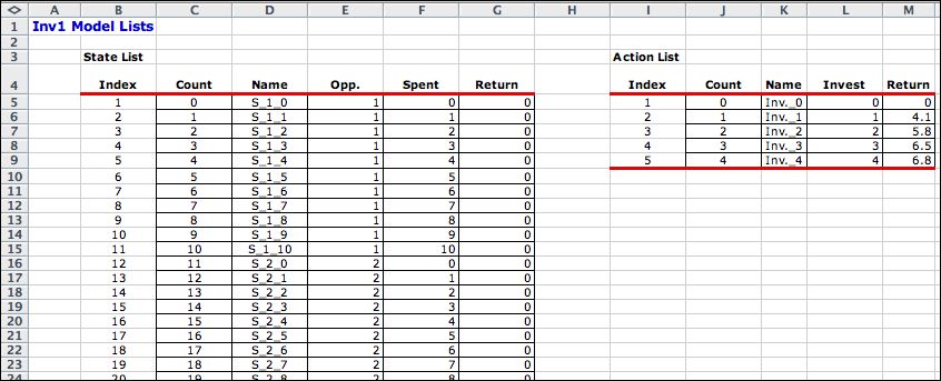
The DP Models add-in
enumerates all feasible states and actions and creates lists
of the elements of the problem. These are transferred to the DP Solver add-in.
The lists are placed on a separate worksheet called Inv1_Lists.
Parts of the lists are shown below. There are 100 states. |
| |

|
| |
 |
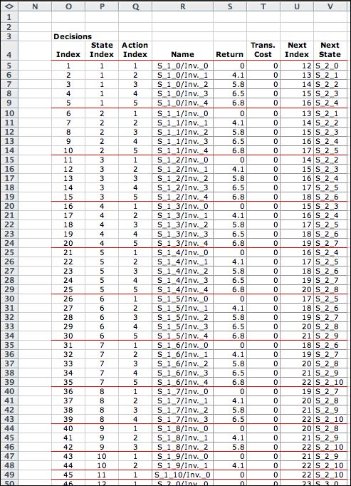
The decision list combines feasible
states and actions that lead to feasible states. There are
372 for this example. Only the decisions relating to states
referring to opportunity 1 are shown. |
|
The DP Solver |
| |
Clicking the Transfer
to DP button, copies the lists to the DP Solver format.
The top left of the DP Solver form is shown below after the problem
has been solved. The acyclic procedure
is useful in a case such as this one, where all states lead
to a state later in the state list. This is called an acyclic
state space. The acyclic procedure starts at the bottom of the
state list and progresses up, evaluating the optimum solution
for each state. Only one pass through the state list is required
for a problem with an acyclic state network. Most deterministic
DP models have this characteristic.
|
| |
|
| |
Part of the solution
is below. The Recover Optimum button at the top of the
page highlights states that comprise the optimum together with
the optimum actions. The value of the optimum policy is 22.3.
The figure shows that 2 units should be invested in opportunity
1, 1 unit in opportunity 2 and 1 unit in opportunity 3. |
|
| |
By hiding the rows for
the states that are not encountered by the optimum, the optimum
solution is clearly displayed. |
|
| |
|
| |
|
|


