|
Some MDP models can
be solved with linear programming. When the discount rate is
not zero, the LP solution determines the limit values of the
NPW. When the discount rate is zero, the results are valid
for a transient systems because the state values converge to
a finite value. |
LP Model |
| |
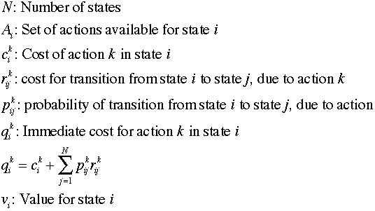
To describe the LP model, we use notation
introduced earlier.

|
| |
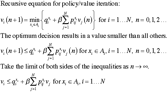
The expressions used for value iteration can
be rewritten as inequalities. Taking the limit with respect
to step number provides a set of linear inequalities.

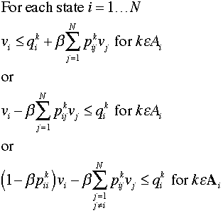
We rearrange terms to show the constant terms on the right
side and the variable terms on the left. The number of constraints
for a given state is equal to the number of alternative actions.

Each constraint has a single positive coefficient
for the column representing the state index. The other terms
are the negative of the transition probability multiplied by
Beta. |
| |
The goal of the LP is to select actions
for each state that will minimize the expected value of operating
the system. We define a probability distribution for the initial
state. The objective is minimize the expected discounted cost
of operating the system over an infinite time horizon.

This objective function plus the constraints
restricting the state values comprise a linear program. Since
the state values may be either positive or negative, we
do not include nonnegativity constraints. |
Example |
| |
We return to the bulb example
to illustrate the LP model. Data from the MDP model relevant
to the LP formulation is shown below. The immediate cost is
the sum of the state cost in column F, the decision cost in
column AC and the expected transition cost in column AD. We
choose the correct value of the state cost using the index
in column Z. The transition probabilities are in columns AH
through AL. There is a row for every decision and a column
for every state.
|
|
| |
With the discount rate of 1%,
the discount factor, Beta, is 0.9901. The coefficients of the
LP constraints and the immediate costs are shown below.

|
Solving the LP |
| |
There is a button at the top of
the DP Solver worksheet with the title Make LP Model.
For this button to be effective the Math Programming add-in
must be installed. The model can be solved with the Excel LP
Solver or the Jensen LP/IP Solver. In the latter case the LP/IP
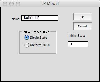
add-in must be installed. Clicking the Make LP Model button
presents the dialog below. A model name is entered on the dialog.
The name shown is the default value for this field. Choose
the initial probabilities by clicking the appropriate button.
The options determine values for the objective function
coefficients. In the first case a single value will be set
to 1 and the others to 0. In the second case, the coefficients
are all 1/N. The coefficients can be changed on the
LP model form.

The LP model for the example is below. The RHS vector holds
the immediate costs. The relationship for each constraint is
<=. Lower and upper bounds to the variables are set to large
negative and positive values respectively. The objective
coefficients reflect the choice of starting the system in
state 1. The constraint coefficients are computed from the
values of Beta and the transition probabilities. |
|
| |
Clicking the Solve button
calls the LP/IP add-in to find the results shown in the range
of green cells. The results are the same as the values
determined with the DP Solver
add-in. The tight constraints indicate the optimum policy. |
|
| |
Sensitivity analysis yields
the dual solution. The nonzero shadow prices for the constraints
1, 3, 5 and 8 indicate the tight constraints and the associated
state/action pairs that determine the optimum policy. Constraint
10 is also tight, but it has a shadow price value of
0. This indicates that the 4-month state is transient for this
problem. Shadow prices depend on the initial state selected
to define the objective function. |
|
Summary |
| |
For the linear programming model of the MDP
the number of constraints is equal to the number of state/action
combinations and the number of variables is equal to
the number of states. Since these numbers are large for many
problems, the resultant LP is often too large for the free
LP solvers available for Excel. More advanced solvers can be
purchased that interact with Excel and solve accordingly larger
problems. For problems with many decisions but few states,
it may be more efficient to solve the dual problem to find
the optimum policy directly.
The LP option for the DP Solver is really not too useful
since larger problems can be solved by the value and policy
iteration methods. The models are interesting for the student
as an alternative to DP. |
| |
|


