|
The analysis
of this and the following pages are for an infinite time horizon.
The model can also be used for finite time horizon problems.
An example is provided later.
The purpose of
optimization in the DP is to discover a policy that results
in the minimum discounted cost of operation of the
system, or the net present worth (NPW), over an infinite
time horizon. The policy prescribes an action for each state.
The optimum policy minimizes the NPW for every state. For simplicity
we call the NPW the value of the state.
The
optimum policy is determined by a dynamic programming algorithm.
The data for the problem is entirely described on the worksheet
created by the add-in. Most of the computations are performed
by equations directly on the worksheet. An iterative process
performed by the add-in implements the dynamic
programming recursive procedure.
On this page we consider the option of evaluating a
fixed policy. Methods on the next few pages find the optimum
policy. |
Value Mathematics |
| |
The DP model is based on states.
The system has a finite numbers
of states. A finite set of possible actions is known, where each
involves some cost that depends on the state and action. Costs
may be negative to represent revenue. Due to the action there
is a transition to another state, the new state may be the
same or different than the current state. There are given probabilities
and costs for the transitions. The events leading to the transition
are mutually exclusive and the transition probabilities sum
to 1. We assume the current state can be observed, actions
are known, and all costs and probabilities are given. Notation
describing these aspects is below.
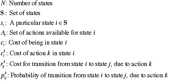
The notation is compressed when we note that
the cost terms can be combined to obtain the expected cost
for an action taken in some state.

For this part of the discussion we assume that
costs expended during future time intervals are discounted
at some positive discount or interest rate d. The discount
factor multiplies some monetary value occurring one period in
the future to find its present worth.

Because the discount rate is greater than zero,
the
discount factor is less than 1. We later discuss the case when
the discount rate is zero and the discount factor is 1. |
| |
A policy specifies a unique action
for each state. We seek the optimum policy.

|
| |
The system is observed at discrete
times. The time horizon may be finite or infinite, but here
we assume that the time horizon is infinite. For the purposes
of dynamic programming we consider time in reverse. Time 0
is the last time to consider. Time 1 is the next to last, and
time n is
the general time (counting backward from time 0). We use subscripts
on our vector notation to describe the states and decisions
at particular times. At any particular time, a value can be
computed that depends on the discounted value for the
next time, the cost of the current state, and the cost of of
the current action. We call these recursive equations. The
value equations below assume that the vector of actions
is given.
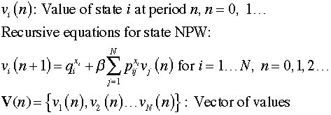
An important assumption of dynamic programming
is that the value of a state depends only on the state and the
sequence of decisions that follow the state. The values for the
states at time 0 must be given. The value at time 1 can then be
computed using the recursive equations. The process continues until
after n evaluations the values at time n are
determined. |
| |
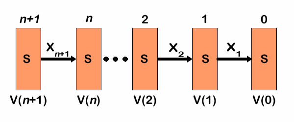
The figure shows a sequence of
values and decisions as time progress in a backward sequence.
Given the values at time to 0 and the sequence
of actions, the values at n can be computed.
The value vector at time n+1 depends only on the value
vector at time n and the actions taken at time n +
1.
|
Probability Mathematics |
| |
When transitions are uncertain,
probabilities can be assigned to the states that depend on
actions and time. When computing probabilities, time
is usually considered in natural order with the system beginning
in some state at time 0. Actions move the system from one state
to another. When transitions are uncertain, a probability distribution
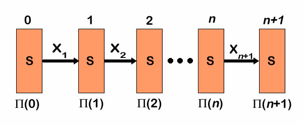
over the state space can be computed. The figure shows the
system starting with some probability distribution specified
for time 0. Transition probabilities determine a different
distribution a time 1, and so forth through time.
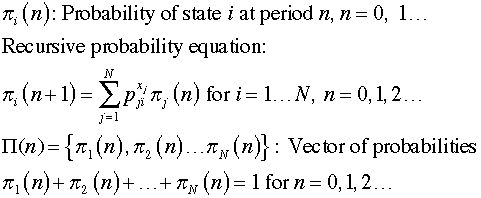
The recursive formula for state probabilities is similar to
the one for values except that
the indices on transition probabilities are reversed. The probability
for state i depends
on the transition probabilities that enter state i.
The DP Solver add-in determines state probabilities
as well as state values. Since the order of computation of
the solver is reversed in time relative to the time sequence
assumed by the probability formulas, the probability values
computed are not correct when the decisions vary over time.
On this page the decision vector is fixed, and it doesn't
matter about the order of computation. The probabilities evaluated
by add-in are correct if one interprets the solver time indices
as the same as natural time.
|
Solution Options |
| |
The add-in has several options
for evaluating given actions and determining the optimum actions.
To see the options, click the Solve button at the top
of the worksheet. The dialog below is presented.
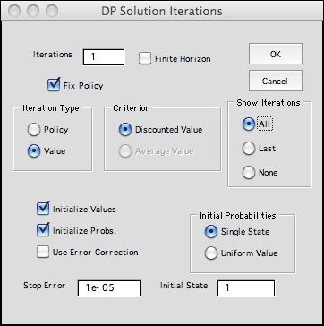 |
The Iterations box
accepts the number of iterations. We choose 1 for the
illustration to show the worksheet with initial values
applied. When checked, the Finite Horizon button
indicates that the problem under analysis has a finite
number of time periods. When not checked and infinite
number of time periods are assumed. The options restricts
some of the features available on the rest of this dialog.
The Iteration Type determines
the solution option. The Policy and Value options
optimize the actions taken from each state. When the Fix
Policy button is checked, the options
evaluate only the current policy. Only value iterations
are available for a finite horizon.
The Criterion specifies the objective of the
optimization. When the discount rate is strictly greater
than 0, the only option is to minimize the discounted
value, or equivalently the NPW of the cash flows.
With 0 discount rate, both options are available, but
the title of the first option is changed to Total
Value.
The Show Iterations options indicate the
intermediate results to be saved. These are placed
on a worksheet called Bulb_DP1_States. With the
All option selected iteration results are saved
from all iterations. With the Last option, only
results for the last iteration are saved. With the None option,
no results are collected, but the final results are shown
on the Solver worksheet. With either the first or second
option, a second dialog box, described in the
next paragraph, determines the information to be collected.
The check boxes at the lower left indicate the whether
the state values or the state probabilities are to be
initialized. When the Initialize
Values button
is unchecked, the current values are used as the starting
point. When it is checked, the final values are determined
by the Final Values column on the worksheet. Some
examples created earlier do not include this column. The
final values are then assigned to be zero.
The Initial Probabilities button determine the starting probabilities
for the analysis. When unchecked the solution uses the current probability
values. When checked, two options are available. The Single State option
assigns the probability 1 to the specified initial state. The uniform
value option assigns equal probabilities to each state such that the probabilities
sum to 1.
The Stop Error fields accepts a small number that causes the program
to termination when an error measure falls below this value. |
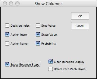 |
On dismissing the iteration dialog with
an OK, the Show Columns dialog asks which columns
are to be included in the display. For present case we
choose to show the action index, state value and probability
value. The checkbox at the lower left inserts a blank column
for each iteration.
The information will be displayed on the columns of
the worksheet. The number of columns for each iteration
is equal to the number of buttons selected (excluding
the two on the lower right). The Excel worksheet is limited
by the number of columns available, and the program will
not proceed if there are so many iterations that the
maximum number of columns is exceeded. |
|
Initial Value Worksheet |
| |
We illustrate the process of value
iterations by showing selected rows and columns of the DP worksheet.
Some are hidden to reduce the width of the display. We concentrate
on the yellow range labeled Discount
Value in
column N and the green range labeled Next Value in row
8. The initial state values are in the range labeled Next
Value. The arrangement of the vector Discount Value in
a column and the vector Next Value in a row simplifies
the calculation. The initial probabilities are in the
range labeled Last Probability.
The figure shows the solver worksheet for the first iteration.
We have chosen the policy to inspect in the first three states
and replace in in months 3 and 4. Column H shows the rows of
the Decision List that determine the policy to be
evaluated. Column H is colored green because the values in
this row are fixed for the analysis. The names for the corresponding
action are in column K. The initial values of 0 are assigned
to the green range labeled Next Value. The initial
probabilities are in the green range of column O. The yellow
range in column N holds formulas that compute the discounted
value after the first iteration. The yellow range in row 9 computes
the state probabilities after one iteration. |
|
| |
With the value option for a fixed policy, we
are solving the equations below for a given action. For
this example, we evaluate the initial action vector (1, 1,
1, 2, 2).

Simultaneously we evaluate the state probabilities.
The initial distribution has the probability of state 1 equal
to 1. The other states have probability zero.

The figure below shows the value computations
when the action vector is fixed at X.

|
Value Iterations |
| |
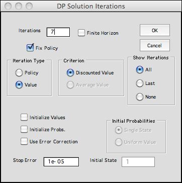 |
Clicking the Solve button allows the analysis
to continue for 7 additional iterations. Since the Initialize
Values and Initialize Probabilities buttons
are not checked, the iterations proceed from the worksheet
obtained for one iterations.
|
|
| |
The results of the iterations
are shown below for 8 steps. The initial solution is shown
in columns I and J. The solution after 1 step is in columns
L through N. The last step, Iteration 8, is in columns AN through
AP. The values are increasing as the iterative process is performed
for more and more steps. The probability vector seems to be
approaching a steady state.


|
| |
Returning to the Solver worksheet
we see the solution after eight iterations. |
 |
| |
Column B shows the results after
8 iterations on the left. The Value Error entry in
row 13 gives a number that estimates the difference between the
current value and the infinite horizon solution. The 127 in this
cell indicates that the values have a long way to go. The Probability
Error in row 14 is computed as the sum of the absolute
differences between the probabilities at iteration 7 and the
probabilities at iteration 8. We call for 92 additional iterations
and the results after 100 iterations are on the right. |
| |
|
|
| The entry in row 13 of the parameter list shows an error
measure that indicates the difference between the value at
the current step and the optimum value. The value difference
is 127.4 indicates that the values have a long way to go..
For probabilities, we sum the absolute differences between
the probability vectors for the current step and the previous
step. The value of about 0.04 shows that the probability
is close to the steady state. |
After 100 steps the value difference is somewhat
smaller. The convergence rate is related to the discount
rate. The larger the discount rate the faster the convergence. The
probability error is effectively 0 after 100 iterations.
The probability estimates do not depend on the discount rate.
For an infinite horizon model, the state probabilities approach
the steady-state value for a Markov chain. |
|
| |
The DP worksheet after 100 iterations
is shown below. The decision indices in column G are colored
green to show the actions are fixed for these iterations. |
|
Error Correction |
| |
Bertsekas gives a method for error
correction in his book (Dimitri Bertsekas, Dynamic Programming
and Optimal Control, Vol 2, Athena Scientific,
2007). The method appears as Proposition 1.3.1 in section 1.3.
We have adapted the method to compute error bounds on the solver
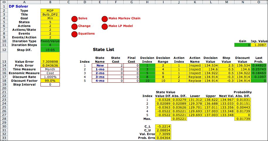
worksheet. The error analysis is placed below the state definition
on the worksheet. The Change button offers the opportunity
to add the analysis to the solver worksheet. The figure below
shows the state portion of the worksheet after 8 iterations.
The value error in cell B13, 7.3, is much smaller than the value
without correction, 127.4. The value vector in column N is much
closer to the infinite horizon solution. |
 |
| |
We request 92 more iterations (for
a total of 100) by clicking the Solve button. The iterations
stop when the iteration counter reaches 37. The value error
has
fallen below the stop error value of 0.00001 specified
on the solver dialog. The value and probability vector are quite
close to those obtained by a Markov Chain analysis of the model
obtained with the fixed solution. Error correction makes a big
difference for many problems. |
 |
| |
This page shows how to evaluate a
fixed policy. The next few pages show how to find the optimum
policy. |
| |
|


