|
The Markov Decision Process (MDP) is solved with the DP Solver
add-in. This is only one of the problem types addressed
by the DP Solver add-in. |
The DP Model |
| |
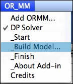
To incorporate actions into the model we select Build
Model from the menu.

|
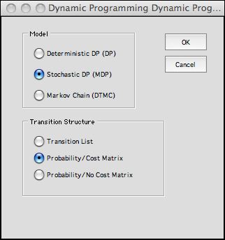
A second dialog asks the type and structure
of the model. We choose to show both the probability
and cost matrix.

|
|
| |
|
Clicking OK presents a dialog
that asks for the parameters of the model to be built.
The fields on the dialog accept the name, number of states,
number of actions, number of events, number of actions
per state and number of events per action.
The column labeled Variables allows
the modeler to associate numerical values with the
states, actions or events, such as those used in the DP
Models add-in. The solver does not use these values directly,
so the zero's shown in this column are appropriate.
The number of actions per state and the number
of events per action determine the size of the Decision and Transition lists.
For the example, each state has two actions: to Inspect or
to Replace.
For each action there are two events: Survive or Fail.
The Make Random Problem checkbox
places random data on the worksheet. This is useful for
illustrating the add-in without data entry. When
the Maximize Objective checkbox is checked, the
add-in constructs a maximization model. Otherwise the objective
is minimized. The goal for the example is
to minimize the expected NPW.
Checking the Include Error Analysis checkbox,
constructs a region on the worksheet where error estimates
and solution modifications are computed. This option provides
faster convergence
in infinite horizon problems. This subject is discussed
later. |
|
| |
|
We illustrate the DP worksheet with several
figures showing selected rows and columns. The cells of
the model are colored yellow, green or white. Only the
white cells hold data that can be directly controlled by
the user. The yellow cells hold formulas and values that
should not be replaced. The green cells hold values computed
by the VBA code. In the following we focus on the white
cells because these hold data for the model.
Columns A and B show the
problem parameters and intermediate results. The content
of the green fields are filled by the solution algorithms.
The bottom three fields can be changed directly by the
user.
Notice
that this example uses a time interval of months and a
discount rate of 1% per month. The discount rate is similar
to an interest rate. The discount factor is the present
value of $1 to be received one time interval from the present.
The discount factor is often given for MDP problems,
so we provide formulas relating the two quantities at the
left. For this model, the discount rate is provided as
data in cell B17. The discount factor is
computed in cell B18.
|
 |
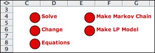
The Solver buttons are to the right of the parameters.
The Solve button
controls the iterations of the DP algorithm. The Make
Markov Chain button constructs
a DTMC model with the current policy. The Change
button allows the student to change the features
of the model. The Equations button
replaces the worksheet equations. This is necessary after
model changes. The Make
LP Model calls
the Math Programming add-in to create a Linear Programming
model of the decision problem. |
|
| |
The data for the problem is placed in
ranges on the worksheet. We have hidden a number of columns
on the worksheet to emphasize
the data rather than the computations.
Columns D through G have state information. Column D holds
the state indices, consecutive integers from 1 through the
number of states. Column E holds the state names assigned by
the user. The State Cost column
holds the direct cost of residing in each state. The Final
Cost column is the costs expended in the final stage of
a finite horizon problem. The
value of 2 in F14 is the cost of the new bulb. It is incurred
whenever the system is in the New state. |
|
| |
Columns Q through S hold the action
data. The Inspect action
expends the cost of inspection, $0.50. The Replace action
results in the cost savings of $0.30 (indicated as a negative
cost). An additional Null action
is provided and may be assigned as an option for some states.
The cost of the Null action is zero. The NA is
assigned when an action for some state is unavailable. The
cost for the NA is very large.
Columns V through X hold the event data. The matrix data
structure does not use the event data explicitly. |
Decision List |
| |
The rows on the worksheet beginning
in column Z and progressing to the right show the decision
list. A decision is a combination of state and action.
Each row shows one state and
one action. For example, row 14 describes state 1 (New)
and action 1 (Inspect). Column Z holds the indices
by which the rows are addressed. Column AA and AB show the
state and action indices respectively. Column AC shows the
names of the state/action combinations.
Observe that each state has two actions, to inspect or replace.
Columns AI through AM hold transition probabilities. These
are important data inputs for any MDP. Even-numbered
rows from 14 through 22 hold the transition probabilities associated
with the inspection option. Odd numbered rows from
15 through 23 hold the transition probabilities associated
with the replace option. This option always brings
the system to the New state. Column AN computes the
sum of the transition probabilities for each row. The sum of
transition probabilities must be 1 for each row and all probabilities
must be nonnegative. Similarly the transition cost matrix has
a row for each decision and a column for each state. All transitions
costs are zero for the example. |
|
| |
The data format showing both transition probability
and cost matrices is convenient for small problems. The number
of columns required by the data is at least 2 times the number
of states. Since the number of columns available on an Excel
worksheet is comparatively small, we provide two more data formats
that require fewer columns. |
Probability Matrix but No Cost |
| |
Given the transition probabilities
and the transition costs it is possible to compute the expected
transition cost for each decision. When this cost is zero or
computed external to the analysis, the cost matrix can be replaced
by a single column. When the Probability but No Cost option
is chosen for the data column AE is provided to hold the expected
cost. This data format uses about half the columns of the option
that includes the cost matrix. |
|
Transition Structure |
| |
This structure is the most efficient
for many problems. Rather than matrices, the nonzero transition
probabilities are described by a list. The decision list no
longer includes the transition probability matrix, but the
transitions are represented by the Expected Transition
Cost vector computed
in column AH. |
|
| |
The transitions are described
in a new list to the right of the decision list called the Transition
List. The example has been modified to include a third
event called New. Each transition is related to a decision
in column AN and an event in column AO. A name in column AP
is a combination of the state, action and event names. Transition costs are
in column AQ, probabilities are in column AR, and next
state indices are in column AS. The Next Name column,
AT, has formulaS that refer to the names in the State list.
|
|
| |
Only transitions with positive probabilities
are listed, so the representation is much more concise than
the matrix options. Most problems have relatively few nonzero
transition probabilities. With the transition list, the number
of transitions is restricted by the number of rows in the Excel
worksheet. The number of columns is no longer a limitation. The
current code is limited to around 32,000 transitions. |
| |
|


