Solution - Value Iterations

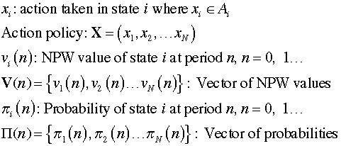
Value iterations find the optimum actions at each step for a finite sequence of steps. As the iterations progress, the policy converges to the optimum for the infinite horizon problem. The state NPW values and probabilities converge to the values for the optimum policy. Several vectors describe the states of the system.

The previous page found the NPW and probability vectors for a specified action policy. On this page we try to find the infinite-horizon optimum policy and the corresponding NPW and probability vectors.

Value Iterations when the Policy is not Fixed

For these iterations the action is optimized at each step. The equation below solves for the optimum action at each state based on the state NPW computed in the previous step. There are N independent optimization problems and each is solved by enumerating all possible actions. The optimum policy is the one that obtains the minimum NPW for each state.

The add-in performs the required minimization with Value iterations. When the Fix Policy button is not checked, the policy is optimized at each iteration. For these iterations we click the Value button on the dialog. The Show Iterations selection indicates whether intermediate results are to be saved. The Final Value and Initial Probabilities options determine the starting conditions for the process. Again we use the Bulb replacement problem for the example.

Step 0 holds the solution with the initial values specified. Note that column G contains indices from the Decision List. The decision list has a row for each state and action combination. For this case there are five states and two actions per state. Thus we have ten rows in the decision list. The transition probability matrix has ten rows and five columns. The indices in column G point to the rows that define the optimum actions for the first step. Thus we see in G14 the index 2, and that row in the decision list shows the action to be 2 when in state 1. The other rows indicated in column G are 4, 6, 8, and 10. We can see from these rows that the optimum is to follow action 2, the Replace action in every state. The optimum depends on the entries in the green range of row 8. These are the initial NPW values specified by the dialog.

By using only the rows specified by the optimum decision index, the matrix of transition probabilities has only 5 relevant rows and 5 columns. This matrix determines unique state values and state probabilities for the initial step.

To make an iteration, the program copies the State Value vector (column M) and pastes the transpose of the values into the vector Next Value (row 8). Similarly the program copies the vector State Prob. (row 9) and pastes the transpose of the values into the vector Last Prob. (column N). The results are shown below.

The program automatically discovers the optimum policy to inspect while in states 1 through 3, and to replace when in states 4 and 5. The optimization step is automatically accomplished with Excel formulas in the yellow ranges of the worksheet. The VBA code of the add-in performs the copy and paste operations described in the last paragraph to implement an iteration.

The program continues through 8 iterations to obtain the sequence of results shown below. The state values and state probabilities change at each step. The policy appears to converge to the policy shown for step 8. Although the values and probability vectors seem to be converging, the results have clearly not obtained the steady-state values.

The values after 100 more steps indicate that the probabilities are very close to steady-state. While the state values are close, they still have not converged to their limit. This is typical with the value iteration process. The optimum action is found rather early in the iteration sequence, however the NPW values take a long time to converge. The probabilities converge rather quickly for most problems.

Markov Chain

The selected rows are transferred into the DTMC matrix. The cost data and discount rate are transferred to the Economics page. After analysis, states 0 through 3 are identified as a single class of recurrent states. State 4 is a transient state. Note that the Markov Analysis indices start at 0 rather than 1 as for the DP Solver page.

Markov Analysis is often useful to analyze the policy obtained with the DP Solver add-in. In addition to steady-state analysis, the Markov Analysis add-in allows several other useful tools. The next page considers the Policy iteration method. This method finds steady-state values that are the same as those obtained with Markov Analysis.