|
For the Policy iteration
method we assume the Markov process is completely ergodic for
every feasible policy. That means that the state probabilities
after a large number of steps are independent of the initial
conditions. This restriction is satisfied for
all the examples considered in this DP section. Most of
the development on this page follows the textbook by Howard
(MIT Press, 1960).
The Policy iteration
method is satisfying because it is guaranteed to return with
an optimum solution, usually with a small number of iterations.
Unfortunately, the method requires matrix inversion to find
steady-state values, and this is only available for smaller
problems. The limit for the policy iteration
method using the DP Solver add-in is 50 states, since the published
maximum size for the Excel inversion routine is 50 rows and
columns. The following vectors are required for the analysis.
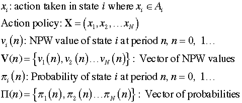
Two methods are incorporated in the DP Solver,
one that is appropriate when the discount rate is positive
and the other when the discount rate is 0. |
Discount Rate Positive |
| |
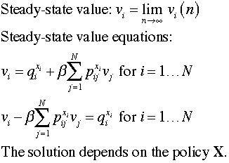
With the value iteration method we noted that
when the discount rate is positive the state NPW values approach
limiting values as the number of iterations increase. Indeed
the absolute differences between subsequent solutions becomes
smaller and smaller as the iteration count grows. Steady-state
NPW values can be obtained by setting the values in subsequent
iterations to be the same. In the following we write equations
for the limiting values of state NPW. By using the limit values
on both sides of the recursive equation, a set of N linear
equations in N unknowns
is identified. Solving the equations obtains the steady-state
NPW values for a particular policy.
|
| |
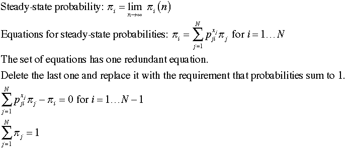
In a similar fashion we compute steady-state
probabilities with the solution of a set of N linear
equations. In this case it is necessary to replace one of
the steady-state equations by the equation requiring the sum
of the probabilities to be equal to 1.
|
Policy Improvement Method |
| |
In this method we start with an arbitrary solution
and find the steady-state values for that solution. Using the
steady-state values we use a policy improvement step to find
a new policy. If the policy cannot be improved, the add-in
stops with the optimum policy. Otherwise, we repeat the steady-state
calculations for the new policy,
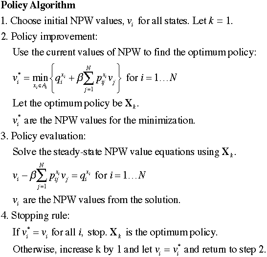
The add-in uses the sum of the difference of
the values used in step 2 to indicate termination. |
Using the Add-in for Policy Iterations |
| |
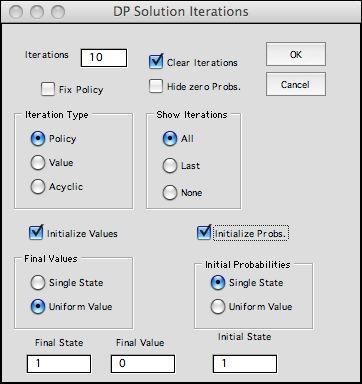 |
Click the solve button at the
top of the DP Solver worksheet and choose the Policy option
from the dialog.
The options at the bottom of the dialog determine
the starting values for the optimization. Although the
algorithm only uses the NPW values, the add-in also finds
steady-state probabilities at each iteration.
|
The figure below shows the initial solution. One column
not shown on previous figures is the Step Value column
L. This is the vector of immediate returns that is used in
the steady-state equations. The replace
action is optimal for all states when the initial NPW values
are set to 0. The formulas on the worksheet automatically
perform the one-step optimization. |
|
| |
The add-in fixes the policy and
solves the steady-state equations for both NPW and probabilities.
The NPW solution is placed in the green cells of row 8.
The probability solution is placed in the green cells in column
N. |
|
| |
The add-in performs the improvement
step to obtain a new policy, inspect in states 1, 2, and
3. States 4 and 5 have the replace action. The steady-state
for this policy has NPW values shown in the green cells
in row 8. The steady-state probabilities are in the green cells
in column N. No improvement is possible and the solution obtained
at the second step is the optimum. |
|
| |
The results of the iterations
are summarized on the worksheet Bulb States, as shown
below.
Step 1 is in columns K though O. Step 2 is in columns Q through
U. The display part of the add-in always repeats the last iteration
in columns starting at C. This makes it convenient to find
the final solution when several iterations are displayed. |
|
| |
These results can be compared
to the values obtained with the Markov Chain analysis for the
optimum solution. The state values (NPW) and the state probabilities
are the same.

|
Matrix Solutions |
| |
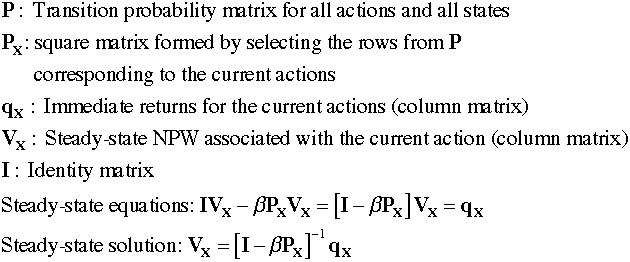
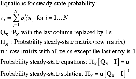
The add-in uses matrix inversion
to compute steady-state NPW values and probabilities. The requirement
of complete ergodicity guarantees that the matrices are invertible.
The matrix equations for the steady-state value solution are
below.
The matrix equations describing the steady-state
probabilities are below.
|
| |
|
The transition probability matrix has 10 rows and 5 columns.
The two rows for each state hold the data for two
actions. A policy chooses 5 rows for the
steady-state analysis. |
|
Policy = (2, 2, 2, 2, 2)
The matrices for
the steady-state analysis are placed below the transition
matrix on the worksheet. The first iteration uses rows
2, 4, 6, 8, and 10 to form the required matrices. The steady-state
NPW solution is computed with Excel formulas in the yellow
range of row AG. The steady-state probabilities are computed
in the yellow range of row 47. |
|
Policy = (1, 1, 1, 2, 2)
The matrices for the second
iteration are constructed from rows 1, 3, 5, 8 and 10.
The results shown are for the optimum policy. |
|
When the Discount Rate is Zero |
| |
When the discount rate is
0, the discount factor is 1. The state values may not converge
as they do for the discounted case. Setting the discount factor
to 1 we find expressions for the total cost as a function of
the step number. For some systems involving a single trapping
state with zero state cost, the total cost does converge to
zero since the system will eventually reach that state. These
are called transient systems. For other systems the cost increases
at each step by a constant that converges to the
average step cost for the system. The values obtained for a
fixed policy with a discount factor of 1 are computed with
the formulas below.

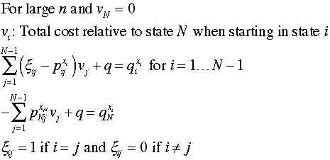
For a large number of steps, the total costs
for sequential steps differs by a constant value g,
where g is the expected cost per step.
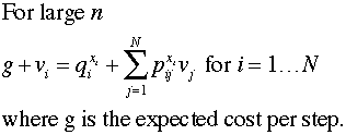
This expression describes a linear set of N equations with
N+1 unknowns, the values for each state and the value
of g. To solve the set of equations, we set the value
for state N to zero. The remaining variables are the
scalar g and
the relative values of the states other than N. In
the equations below, we have rearranged the variables so that q is
the last variable and the immediate returns are on the right
side. The coefficients of the relative costs are the negative
of the transition probabilities except for the diagonal term
that has the coefficient of 1 less the self-transition probability.
The following figures show the sequence of solutions
with the policy method when the discount rate is 0. The first
figure shows the initial solution. The green range in row 8
starting in column AH is the state values relative to state
5, v(0). The values in the yellow range of column
M are v(1). |
|
| |
The first step evaluates the initial
policy. The state values in column M are the steady-state costs
when the policy is to replace the bulb at every age. The cost
depends on the initial state. |
 |
| |
The improvement step finds that it
is optimum to inspect at ages 0, 1 and 2 months, but replace
at months 3 and 4. The steady-state values and steady-state
probabilities are in columns M and N for this solution. |
 |
| |
At this step, no improvement is possible
and the process terminates.
At each step the entry in cell M10 is the value of g computed
with the solution of the linear equations. The value in cell
N11 is the expected values of the step value vector using the
probabilities computed in column N. The contents of M10 and
N10 are computed with different processes, but they are the
same. In the figure they appear different because column N
is a little wider allowing one more significant digit.
We repeat the steps of the analysis below showing the matrices
and solutions. |
| |
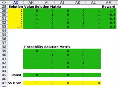 |
Policy = (2, 2, 2, 2, 2)
The matrices for the steady-state analysis are placed
below the transition matrix on the worksheet. The first
iteration uses rows 2, 4, 6, 8, and 10 to form the required
matrices. The 1's in column AL are the coefficients of
the gain, g. The relative total cost solution
is computed with Excel formulas in the yellow range of
row AG. The steady-state probabilities are computed in
the yellow range of row 47.
The value of g is in cell AG33. |
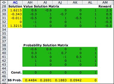 |
Policy = (1, 1, 1, 2, 2)
The matrices for the second iteration are constructed
from rows 1, 3, 5, 8 and 10, substituting 1's for the last
column of the Value Solution Matrix. The results shown
are for the optimum policy. |
|
Summary |
| |
The policy iteration method is convenient because
it solves for the optimum solution and the resultant state
values and probabilities. When the discount rate is positive,
the policy iteration method finds the optimum NPW value for
each state and the optimum policy. When the discount rate is
zero, the policy method computes the value of g as
well as the relative state values for all the states. The add-in
automatically uses this form of the policy method when the
discount rate is very small.
The
disadvantage of policy iteration is that it requires matrix
inversion. The Excel inversion function is limited
to 50 variables. Experiments with Excel 2007 indicate that
this may not be a strict restriction because problems with
more than 50 states have been solved. Excel 2003 for PC's and
Excel 2004 for Macs are currently limited to 50 variables.
|
| |
|


