We illustrate this case with the aggregate scheduling problem described in the modeling section. A company wants a high level, aggregate production plan for the next 6 months. Projected orders for the company's product are listed in the table. Over the 6-month period, units may be produced in one month and stored in inventory to meet some later month's demand. Because of seasonal factors, the demand for the product and the cost of production is not constant, as shown in the table.

The cost of holding an item in inventory for 1 month is $4/unit-mo. Items produced and sold in the same month are not put in inventory. The maximum number of units that can be held in inventory is 250. The inventory level at the beginning of the planning horizon is 200 units; the inventory level at the end of the planning horizon is to be 100. The problem is to determine the optimal amount to produce in each month so that demand is met while minimizing the total cost of production and inventory. 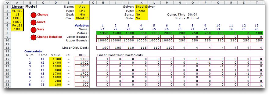Shortages are not permitted. The general model is below.

We construct the model with the Math Programming add-in and solve it with the Excel solver to obtain the solution below.

Using the Side Model

In the formulation above one notes that the constraint matrix is sparse, that is, it contains many 0's. This is usually true in a multiperiod model because most of the variables appear in the constraints associated with only a single period. For this simple example there is only one constraint per period. Each production variable is present in only one constraint while each inventory variable appears in two. We will construct a more compact model using the side model feature. For this purpose we identify the inventory variables as the linking variables in the master problem and the production variables as the side variables in the subproblems. First we construct the master problem shown below. Only the inventory variables are included with the two constraints describing the beginning and ending inventory. The solution to the model has no meaning since important information regarding demand and production cost is not included.

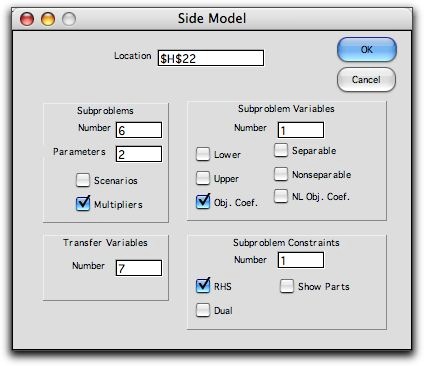
To create the subproblems. choose Side Model under the Math Programming add-in entries in the ORMM menu item. The dialog below contains the parameters of the side model.

The cell field indicates the location on the worksheet for the side model. Replications is the number of rows, or individual subproblems to construct. Parameters indicates the number of columns to include with model related parameters. Transfer is the number of linking variables. Variables is the number of side variables in each of the subproblem rows. The Obj. box indicates that a column is to provided for objective coefficients of the side variables. Constraints indicates the number of constraints for each row of the side model. The RHS box indicates that a row is to be included for the Right-hand-side values. Clicking OK results in the side model below. The formulas shown in row 19 link the data in the parameter columns to the objective and RHS columns.

The T and W matrices are composed entirely of 1's. The D rows determine the contribution of the master transfer variables to the constraints.The constraints described by the side form are:

z0 - z1 + x1 = 1300
z1 - z2 + x2 = 1400
z2 - z3 + x3 = 1000
z3 - z4 + x4 = 800
z4 - z5 + x5 = 1700
z5 - z6 + x6 = 1900

The model form includes a Change button that allows columns of the side model to be added or deleted. Addition of columns is possible only if the associated region currently has at least two columns of that type. In the example, the numbers of parameters and transfer variables can be increased, but the number of side variables and side constraints cannot.

When we click the Solve button at the top of the page. The solution to the combination of the main model and the side model is obtained. The solution is the same as when all the variable and constraints were included in the same model.

Adding Fixed Charges

For such a simple problem, there does not seem to be a very large savings when using the side model, rather than including the entire problem in the master problem. More savings are apparent when the side model grows in size. For an example we change the problem to add a fixed charge whenever nonzero production occurs. The fixed charge might represent the setup cost for producing a product.

The master problem shown below is the same as the original except we have increased the maximum inventory to allow a more interesting solution. The figure shows the optimum solution