The side model can only be used if one of the other model forms, linear, nonlinear, network flow or transportation, has already been constructed on a worksheet using the procedures described earlier in the Math Programming section. We call the problem described by the original model the master problem.

The side model is a series of one-line models. The one-line models are called subproblems. Each subproblem occupies cells on a single row of the Excel worksheet. Cells on the row contain all the variables and constraints for the subproblem as well as parameters and coefficients sufficient to define the model. The side model can have a large number of rows to represent a whole series of similar subproblems. The subproblems are linked to the original model by variable values transferred by equation from the master problem. We will see that a very large model can be constructed with a relatively small number of cells on the worksheet. We can use the Excel Solver to solve these problems, but only models of very limited size can be solved with the free Solver available with Excel. The Jensen LP/IP Solver has recently been modified to implement the L-Shaped method so that quite large models may be addressed. The L-shaped method is a decomposition method for solving problems with side constraints.

The side models are very useful for stochastic programming models, models that involve piece-wise linear approximations and models that include fixed charge variables. Several examples are presented in the first three pages. The L-shaped method is on the two remaining pages.

The Block Diagonal Form

An LP is presented below with the form that suggests that a side model might be useful. In the figure below, the colored regions in the constraint coefficients may contain nonzero numbers, while the cells outside these regions contain all zeros. The constraints of this model have the block diagonal form. There is a set of variables x that are related by the first two constraints through the matrix A. The variables in z are also included in this set of constraints via the matrix A'. The following six constraints contain z and the variables labeled y11, y12, etc. In the following we call these variables yk where k=1, 2 or 3. These constraints contain nonzero coefficients in the matrices T and W. The constraints can be divided into sets so that y1 appears in the first, y2 appears in the second, and so on. The matrix T multiplies z in each set, and the matrix W multiplies yk. The lower bounds, upper bounds and objective coefficients are similarly partitioned. The RHS values of the constraints are also partitioned in this fashion into b, d1, d2 and d3.

The full matrix representation of a problem with the block diagonal form is not efficient because of the large number of zero's in the matrix. Although 0's do not affect the efficiency of the Solvers significantly, the large matrix consumes many cells of the Excel worksheet. The number of cells grows as the product of the number of variables and the number of constraints. Entering the nonzero data is difficult because it is hard to keep track of rows and columns. In the form presented, the number of variables is limited to the number of columns of the worksheet (the maximum is about 250). Numbers associated with data lists outside the form are not identified with regard to source thus making the model difficult to check and maintain. These difficulties magnify as the number of blocks in the diagonal form increases.

The form is also called the L-Shaped form because the nonzero entries roughly resemble an inverted L. The matrix A comprises one bar or the L, while the matrix to the right of A comprises the other bar.

Side Model

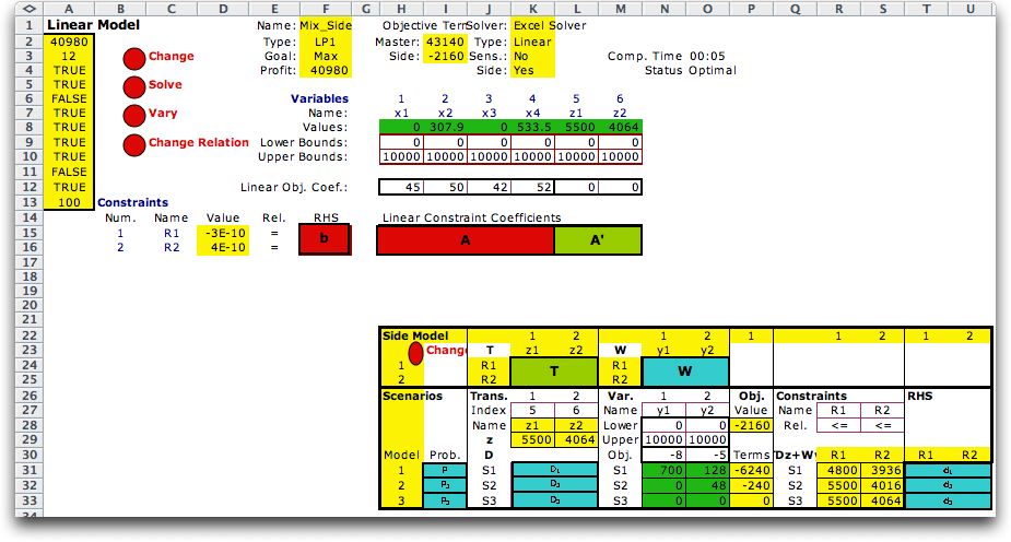
The side model shown below provides a more efficient representation that does not include all the 0's. The model at the top of the page (through row 16) is master problem. It describes the first two constraints with the variables x and z.

The side model starts in row 22 and contains the information describing the subproblems. The linking variables, z, and the associated matrix T is in columns J through L. The linking variables are identified by the indices in cell K27 and L27. The names and values of z1 and z2 are transferred through equations in the range K28:L29. The subproblem variables, bounds and objective coefficients and the matrix W appear in columns N and O. The variable values are in the green range N31:N33. These are determined by the Solver. The objective function for the side model is computed in column P. The objective terms are weighted by the numbers in column I. The constraint values, names and relations are in columns R and S. The RHS values are in columns T and U.

At the top of the page we see the objective function contributions of the master and subproblems in cells I2 and I3 respectively. These are totaled in cell F4. The value of cell F4 is maximized by the Solver.

Notation

The options are more easily discussed when we define notation for problems with the block diagonal form. The general problem is at the left. The model expressed with subproblems is at the right. For simplicity, the forms are shown with equality constraints, however, they can be expressed as inequalities as well. We show all lower bounds to be zero, but the forms allow nonzero or negative lower bounds. We show a linear programming model, but the side model can also be attached to nonlinear master problems, network flow models or transportation models. The side models may include nonlinear terms in the objective function.

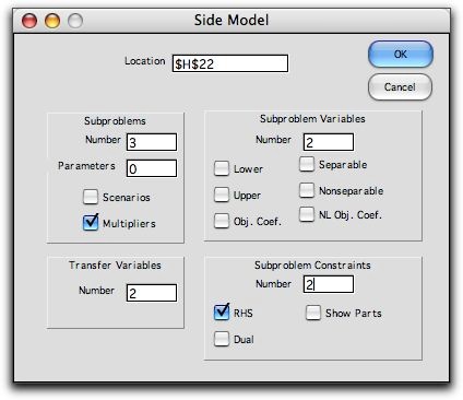
After a master problem has been placed on a worksheet, a side model is constructed by selecting the Side Model item from the Math Programming menu. The dialog below is presented.

The dialog presents options that determine where the side model is placed on the worksheet and the features that are to be included as specific data columns. The cell at the upper left corner of the side model display is indicated in the Cell field. The Subproblems field holds the number of subproblem rows to be included in the side model. Parameters indicates how many columns are to be included to hold parameters of the subproblems. It is often useful to have all relevant parameters entered in these columns, but the parameters can be entered directly in the data columns describing the subproblems. Transfer is the dimension of the linking variables z. Variables is the dimension of the subproblem variables yk. The Constraints field holds the number of constraints in each side problem. The buttons Lower, Upper, and Obj indicate whether specific columns are to be dedicated to these values. If not checked the values are provided by single cells that pertain to all the subproblems. Separable Nonlinear includes columns for separable objective function terms and their coefficients. Nonseparable Col. includes a column for nonseparable nonlinear terms. RHS button includes a columns to hold a different RHS value for each subproblem. Otherwise a single value is provided to pertain to all subproblems. The Show Parts button provides a column for the value of TDkz another for Wyk. We illustrate a variety of options in the example problems that follow.

Although the example shows a common matrix T for all subproblems, it is often useful to have different matrices for the different subproblems. This is provided by the matrix Dk that varies by subproblem. In matrix notation, Dk is a diagonal matrix that multiplies T. The effect is that the transfer matrix can then be varied by subproblem. Since only the diagonal elements are relevant they are stored on our form in each subproblem row. Although not every situation can be handled using these matrices, we will find that they are very useful for some applications. For applications that have a constant transfer matrix T, the values in the cells are all set to 1. Then D is an identity matrix.