We have statistical data that relates some dependent variable to one or more independent variables. With multivariate regression we seek an expression that explains at least some of the variation of the dependent variable by a function of the independent variables. An example is provided in Barnes. We have 13 observations of the value y with corresponding values of x1 and x2.

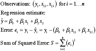
We seek a relation involving the two independent variables that estimates the dependent variable. The estimate is and the relationship is linear with respect to the unknown Betas as shown below.

One criteria for choosing the Beta values is to minimize the sum of squared errors. The resultant expression is called the least squares fit. There are matrix formulas that give closed form expressions for the Betas, but on this page we use math programming to solve the problem. The math programming model is below.

For the example n is 13. There are 16 variables for this problem, three Betas and 13 error values. There are 13 constraints. When the constraints are satisfied, the errors equal the difference between the observed values and the estimates. The objective is a nonlinear quadratic function.

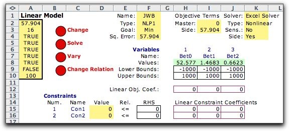
This model is most easily setup using the side model feature. The master problem simply defines the Beta variables and provides them with unrestrictive bounds. The program requires at least two constraints for the master problem, and the 0 coefficients make the constraints meaningless. The results shown are from the optimum solution.

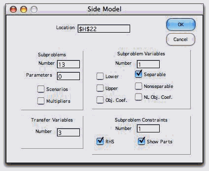
The remainder of the model is provided by the side model. There are 13 subproblems, one for each observation. We click the Separable button to provide the squared terms of the objective function. The RHS and Show Parts buttons are also checked.

The model below has all the features required. The x1 and x12 values appear as the coefficients of Bet1 and Bet2, respectively (columns K and L). The coefficients of the constant term is 1 for all observations (J). The observed values are placed in the RHS column (T). The variables of the subproblems are the error values, e in column N. These values, shown with a green background, are the results of the optimization. Their values are determined by the equality constraints in column S with RHS values in column T.

The nonlinear features of the problem are provided in column P. The pink cells of the column hold equations that square the numbers in column N, thus obtaining the mean square error. The linear terms in column O do not affect the solution because of the 0 coefficient in cell N29. By using the Show Parts button, the information in columns U and V are included. Although not necessary for the solution, these columns explicitly show the estimates in column U and the errors in column V. The solution shown was determined by the Excel Solver to minimize the objective function which is the sum of the squared errors. This is the same solution as obtained by Barnes with the traditional matrix methods.

For a second example of regression we consider the problem of fitting a polynomial in the independent variable. The data below shows 21 values of an independent variable, x, and observations of a dependent variable, y.

We hypothesize that the value of y is related to the value of x through a polynomial of x, however, the relation is not exact. We want to find the coefficients of a fifth order polynomial that minimizes the sum of the squared errors.

This problem has 26 variables, six a coefficients and 21 error values. There are 21 constraints, one for each observation. The polynomial coefficients are defined in the master problem. The ranges for the coefficients are set as the lower and upper bounds of the variables. The green range in row 8 shows the optimum coefficient values.

The side model defines the error variables in a single column (S). Lower and upper bounds are in cells S27 and S28. The solution describes the optimum polynomial coefficients and the associated errors. Again this is a nonlinear optimization problem because we are minimizing the sum of the squared errors.

Absolute Value Error

An alternative criterion for a regression problem is to minimize the sum of the absolute values of the errors. The math programming model for this problem includes variables for the positive and negative deviation between the observed and estimated curves. The resultant model is a linear program.

Here the error is divided into two parts as the positive and negative deviations from the estimated lines. The absolute error is the sum of the two parts. At optimality at least one of the positive or negative deviations will be zero for each observation. The Excel model has the same master problem, but the side model has two variables for each subproblem. The worksheet below shows the coefficient estimates as well as the errors.