The L-shaped method is a decomposition method that is useful for solving problems that have the form of a master problem and several subproblems represented by the side model. The complete problem with both the master and subproblems may be very large and beyond the capabilities of the available Excel solver. The L-shaped method is a process that solves a sequence of much smaller problems. The combined solution converges in a finite number of iterations to the optimum. Because the number of required iterations may be large, we can terminate the process when the lower and upper bound values differ by a specified minimum tolerance. We have implemented the L-shaped method in the Jensen LP/IP Solver. This page describes the application of the method while the next page discusses the theory.

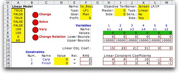
We illustrate the method with the small problem used to introduce the side model for stochastic programming. The Master problem is below. The Jensen LP/IP add-in is identified as the solver. A larger illustration is the Capacity problem in the stochastic programming section.

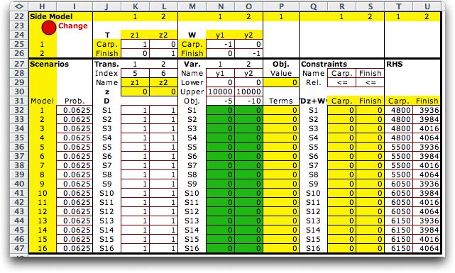
There are 16 scenarios for the stochastic programming model represented on the side model. An important restriction to this method is that all subproblems be linear programs. This makes nonlinear or integer forms inapplicable. Also the subproblems must have feasible solutions for every feasible solution for the linking variables. It is always possible to create models for which this is true, but the method will terminate if a subproblem happens not to have a feasible solution for some solution for the linking variables encountered during the solution process.

Clicking the Solve button at the top of the page (not the one in the side model form) presents the L-Shaped algorithm dialog.

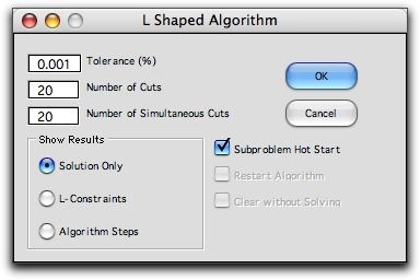
The fields at the top of the form are parameters for the method that will become meaningful as the example progresses. The buttons at the bottom indicate how much of the solution process is displayed. The Solution Only button solves the problem and then eliminates all intermediate information from the worksheet except a Lower Bound (or Upper Bound) cell just below the objective value. The L-Constraints button shows the extra constraints added to the master problem by the method. The Algorithm Steps button stops the algorithm at each step of the process so the student can review the current status and perhaps terminate the algorithm.

The Subproblem Hot Start checkbox solves the series of subproblems more rapidly by solving each subproblem (after the first) starting with the optimum basis for the previous subproblem. Except for very small problems, this results in faster computation times. We allow the option to be unchecked in case the hot-start is not effective. Solving the problem with the options above results in the solution below.

Optimality Cuts

By selecting the L-Constraints option on the dialog, we see the additions to the master model during the performance of the L-shaped method.

The method consists of several iterations. Except for the last, each iteration adds a new constraint to the master problem that restricts the set of feasible values for the linking variables, in this case z1 and z2. They are called Optimality Cuts because they cut-off solutions that cannot be optimal. As the iterations progress the upper and lower bounds grow together. When their difference is smaller than the specified tolerance, the process stops and presents the best feasible solution found. For the present example the best is also the optimum.

The constraints are added from the bottom up. Thus the constraint labeled Opt1 was the first, and the constraint labeled Opt5 was the last.

As new optimality cuts are added, old cuts may become loose. Although there is no guarantee that cuts that become loose at one iteration will not be binding for a later iteration, it is common practice to limit the total number of cuts included in the model simultaneously. The dialog allows a separate input for this purpose. When the number of simultaneous cuts is fewer than the total number of cuts, it is possible that the method will take more iterations or even fail to converge. On the other hand, with fewer simultaneous cuts the LP model for the master problem will have fewer constraints and be easier to solve.

The method may be restarted with new parameters by clicking the Restart Algorithm checkbox.

Algorithm Steps

For the student or teacher interested in the steps of the algorithm, we provide the Algorithm Steps button.

At each iteration a dialog is presented at the top of the worksheet with the current upper and lower bounds. The master problem on the worksheet can be seen behind the dialog. The constraint at the bottom of the model is the optimality constraint determined by the solution to the subproblem. The constraint is violated. In the second step the solution must satisfy the new constraint. The figures below show the five steps required for the example.

Clear without Solving