|
The traditional traveling salesman
problem involves a salesman who must make a route through some
set of cities. Starting at an arbitrary city, the salesman must
visit the other cities and then return to the starting city.
The distance between every city pair is specified and the salesman
is to visit each city once and only once. A solution is called
a route and the goal is to find the minimum length route. This
problem is considered by the Optimize add-in. A new add-in,
the Routing
add-in has a more extensive model for the routing problem. |
|
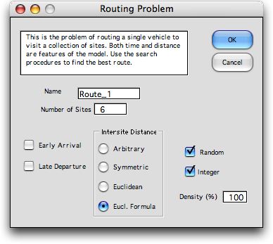
The routing problem
addressed by the Combinatorics add-in
is similar to the TSP, but here we are dealing with a
vehicle that starts at a depot, visit several sites and
returns to the depot. The objective is to minimize the
travel cost plus a cost that depends on the
delivery times to the cities. The parameters of the problem
are set in the dialog below.
|
|
| |
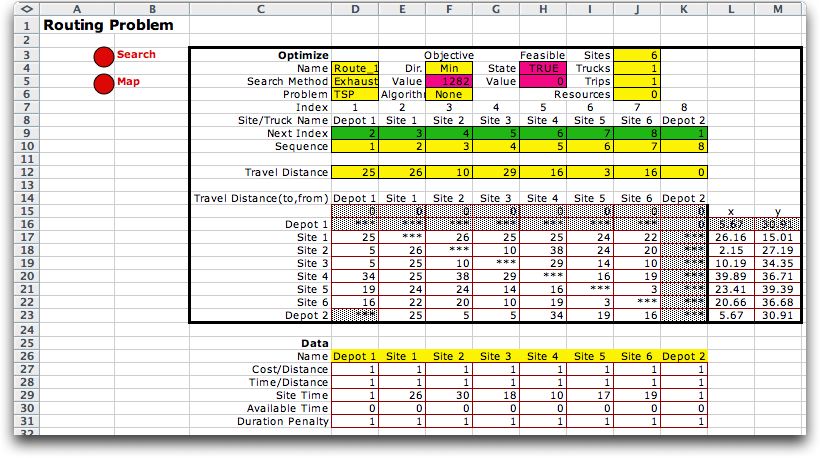
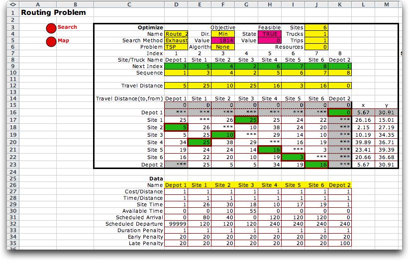
Features of the problem are illustrated
by the example. Two additional sites are defined for the analysis.
The site indexed 1 represents the depot at the start of the
route, the site indexed 8 represents the depot at the end of
the route, and the six specified sites are indexed 2 through
7.
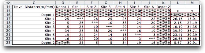
Time is the essence of this problem. A distance matrix (rows
16 to 23) describes the distances between each pair of sites.
Note that entry (i, j) holds the distance
to site i from site j. This is different
than the usual definition, but more convenient for modeling.
Since the random, Euclidean and integer options were specified,
the locations of the sites are randomly generated and shown
in columns L and M. The first and the last sites both represent
the depot and they have the same location. The Euclidean distances
between the site locations are computed and the integer portions
of the values are placed in the table. If the Euclidean
Formula option
had been chosen, Excel formulas evaluate the distances. The
user can then provide non-random locations for the sites in
columns L and M. If a density less than 100% is chosen cells
are randomly selected to hold a numeric value with the specified
probability. The remainder of the cells are made inadmissible
by placing the string "***" in them. The add-in assures
that at least one feasible route exists.
Since the route must start at Depot 1, all cells allowing
a transition from a site other than the last site are disallowed.
Similarly all cells representing a transition from the last
site to other sites, except the first, are disallowed. Also
the cell from Depot 1 to Depot 2 is disallowed. The cell from
Depot 2 to Depot 1 completes every feasible route. The grayed
cells in the table have values necessary for the add-in and
should not be changed. Although the other cells are computed
with formulas, their contents can be changed to more accurately
reflect travel distances.
Refer to the figure below for the remainder of the discussion
about the example. Distances are translated into costs by cost/distance factors
(row 27), and into time by time/distance factors (row
28). The vehicle must spend time at each site, perhaps for
loading and unloading, called the site time (row 29).
There is also an available time (row 30) for each
site that is the earliest time a site can accept the arriving
vehicle. The objective in this problem is to minimize the cost
associated with the route. The duration penalty (row
31) multiplies the departure time from each site to determine
the cost of the route. Early and late costs may also be included
as described later.
The sequence of sites visited by the vehicle is called a route.
The route begins at the depot and ends at the depot. The initial
default route follows the sites in numerical order as in row
10. The decision variables for the problem are in row 9. An
entry specifies the next site to visit from the site associated
with that index. For example, the solution shown starts at
site 1 (the depot) and the next index is 2 (site 1). The route
is computed from these decisions and shown in row 10. Row 12
shows the travel distance from a site to the next site in the
route. |
|
Evaluation |
|
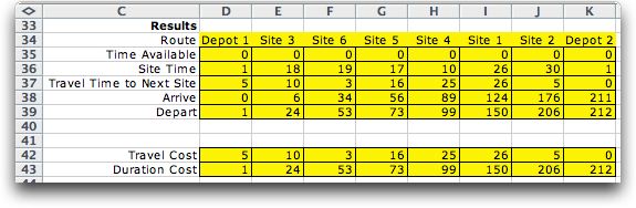
Immediately below the data, the
sequence is evaluated. All these cells are yellow indicating
that they are determined by formulas. The current sequence
of site visits is in row 34. The Time Available and Site
Time values are gathered from the data and presented in
the order of route sequence in rows 35 and 36. The Travel
Time to Next Site values in row 37 are computed by multiplying
the travel distance by the Time/Distance values
in the data. The Arrival Times are in row 38 and
the Departure Times are in row 39. The arrival time
for a site is the maximum of the time available for the site
and the sum of the departure time of the previous site and
the travel time. The departure time for a site is the sum of
the arrival time and the site time. The arrival time for the Depot shown
in column D is the time available value for the depot. The
arrival time for the Depot shown in column K is the
time required for the completed route.
The cost information begins in row 42. A Travel Cost in
row 42 is
obtained by multiplying the travel distance by the Cost/Distance data
item in row 27. A Duration Cost in row 43 is computed
by multiplying the departure times in row 39 by the Duration
Penalty in row 31. The sum of these costs are reported
in cell F5 at the top of the page. The goal is to find a sequence
that minimizes this value.
When the duration penalties are zero, the travel cost is minimized
by minimizing the total distance traveled on the route. This
is the familiar traveling salesman problem. Nonzero duration
penalties penalize a delivery in proportion to the time the
route departs from the site. Thus time is important in addition
to distance. Preference between sites can be expressed by using
higher penalties for sites of higher priority.
When all penalties
are the same, the route will tend to serve sites with short
durations earlier than longer ones. For example if the Cost/Distance values
are set to zero, the tour will follow the shortest time rule,
serving the sites with the smallest site time first. Since
the objective is the sum of the distance and time effects the
optimum tour will balance duration penalties with travel costs. |
| |
|
Optimization |
| |
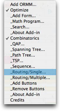
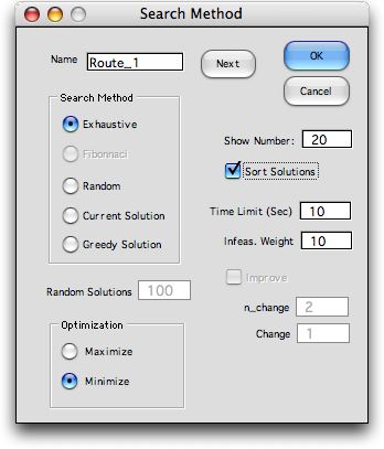
We choose a solution method by clicking the
Search button on the worksheet. The button calls a
dialog from the Optimize add-in for selecting the
solution method. The dialog shows the Exhaustive search
method chosen. The 19 best solutions are to be shown in a
sorted list. The best solution found appears twice in the
list.
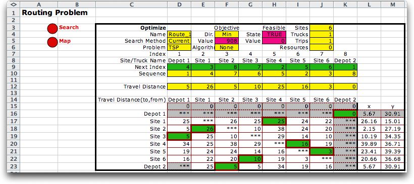
The figure below shows the worksheet with
the optimum solution found with exhaustive enumeration. The
cells defining the optimum route are outlined in red on the
distance matrix. Of course, any other method besides exhaustive
enumeration does not necessarily provide the optimum solution. |
|
| |
The route results are shown below.
The route follows the sequence (Depot, 3, 6, 5, 4, 1, 2, Depot).
The minimum total cost for the data provided is 908 (in cell
F5). |
|
| |
When x and y coordinates
are given in the data graphical
display of the route is also available. Clicking the Map button
creates a worksheet showing the route. Some data formats do the
provide the coordinates, so the Map option will not be available. |
|
| |
The list below shows the best 19
solutions found by exhaustive enumeration. The optimum solution
was also found by generating 10 random routes and improving each
with a 2-change heuristic. Of course, such a fortuitous result
cannot be guaranteed. Note that the solutions do not give the sequence
directly. Rather the solution provides the next site to
visit from each site. The associated sequence for for a solution
can be found by placing the solution in the green area on the
problem form, row 9 in the example. |
| |
|
Scheduled Arrival
and Departure Times |
| |
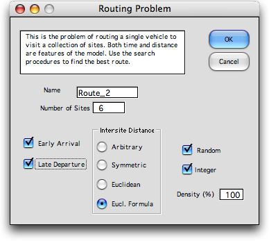
To include scheduled arrivals and departures
in the data, click the Early Arrival and Late
Departure checkboxes. For this example, we construct the
distance matrix with formulas determining the Euclidean distances.
|
| |
The form for the example is shown below with
data. With the Early Arrival and Late Departure options,
some new data rows are provided. There is now Scheduled
Arrival (row 30) and Scheduled Departure (row
31) data for each site. Early Penalty (row 33) and Late
Penalty (row 34) values penalize deliveries that are earlier
than the scheduled arrival time and later than the scheduled
departure time.
The data below requires
that the vehicle finish its route before 240 minutes
or 4 hours. Sites 1, 2 and 3 have been promised that the departure
times will be no later than 120 minutes. Sites 4, 5 and 6 have
been promised that the vehicle will arrive no earlier than
120 minutes and that departure will be no later than 240 minutes.
To encourage a completion time for the entire route of 240
minutes, we have placed 240 as the scheduled departure from
the final depot site. Scheduled arrivals and departures are
soft constraints. We encourage them to be satisfied by penalizing
arrivals that come before the scheduled times and departures
that occur after the scheduled times. A greater penalty is
applied to the last depot site to give greater priority to
the desired route completion time.
The data also specifies that site 2 will be available no earlier
than 10 and site 3 will be available no earlier than 55. These
are hard constraints. |
|
| |
Clicking the search button at the top left of
the page, we choose Exhaustive as the search option.
The solution above is the optimum solution.
The results below
describe the optimum route. The optimum sequence has site 2
(index 3) as the first site on the route. The vehicle arrives
at time 10, when the site is first available. This is 30 minutes
before the schedule arrival resulting in a penalty of 600.
The second site on the route, S3, is within the scheduled time
window. The departure time for S1 is 4 minutes after the scheduled
departure time resulting in a penalty of 80. The entire route
is finished at 231 minutes, within the desired limit. |
| |
|
| |
Clicking the Map button on the page
causes a worksheet to be created that shows the solution graphically.
Note that the route is different than the example without early
and late times. |
|
| |
The single vehicle routing problem with time windows modeled
here is just one of the many vehicle routing problems that
could arise in practice. Many varieties have been considered
in the literature including problems involving more than one
vehicle and vehicles with finite capacities. These are also
combinatorial problems but they involve a more complex decision
structure than the simple sequencing considered on this page.
The add-in is generalized for the multiple vehicle case on
the next page.
|
| |
|