|
|
 |
Combinatorics |
 |
-Quadratic
Assignment Problem |
| |
To illustrate the add-in we consider
a small problem described by Ronald Rardin in his book Optimization
in Operations Research. The example illustrates a location
problem, one of the applications of the QAP. Another example
is found in the section on Facility
Layout.
A small shopping mall has four shop locations. The walking
distance, in feet, between all pairs of locations are shown
in the table below.
Distance |
1 |
2 |
3 |
4 |
1 |
0 |
80 |
150 |
170 |
2 |
80 |
0 |
130 |
100 |
3 |
150 |
130 |
0 |
120 |
4 |
170 |
100 |
120 |
0 |
Four shops, designated A, B, C and D, are to be assigned to
the four locations in such a way that customers traveling between
pairs of shops will not walk too far. We have data on the number
of customers per week that travel between the shops. The data
is shown in the table below. The entries are in thousands of
trips. We show the trips in the upper diagonal of the table
although the trips might be in either direction. Although the
program can handle directional travel, the distribution of trips
between the two directions doesn't matter for a symmetric distance
matrix.
Trips |
A |
B |
C |
D |
A |
0 |
5 |
2 |
7 |
B |
0 |
0 |
3 |
8 |
C |
0 |
0 |
0 |
3 |
D |
0 |
0 |
0 |
0 |
The problem is to specify a location for each department. Call
x(i) the location assigned to department i
and say that there n departments (and locations). The
distance between two locations, say k and l,
is d(k, l) and the flow between two
department, say i and j, is f(i,
j). The trip-distance contributed by departments i
and j to the objective function is:
f(i, j)*d(x(i),
x(j))
Summing over all department pairs provides the
QAP objective function:
Sum(i = 1…n)[Sum(j
= 1 to n, i <> j){f(i,
j)*d(x(i), x(j))]
We will see that this objective is efficiently
represented using Excel functions. |
Creating a Model |
|
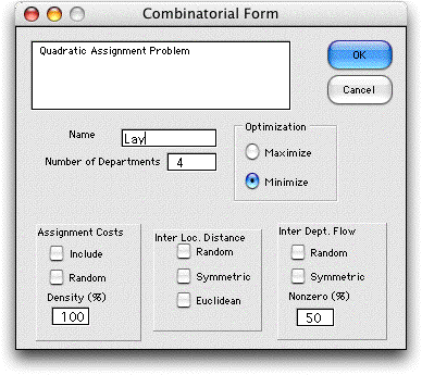
To create a model, we choose
the QAP command from the menu. The dialog accepting
the parameters of the model is presented.

For the example, we enter 4 as the number
of departments and specify a name for the problem. As usual,
this name should be short and it must not include spaces
or punctuation. The name provides the worksheet name and
is the prefix for a number of array names on the worksheet,
so once specified, it cannot be changed. We choose to minimize
the objective. The check boxes at the bottom of the dialog
determine whether assignment costs are to be provided and
whether random data are to be placed in the problem arrays.
The add-in creates a worksheet with the name Lay and
calls the Optimize add-in to create a permutation
combinatorial form. We have entered the interlocation distances
and the interdepartmental flows into the matrices constructed
by the add-in. The initial solution assigns the locations
to the departments in numerical order and places the solution
in row 9. |
|
| |
|
| |
We see a third matrix, the Sorted
Distance matrix, at the bottom of the form that plays an
important role in the model. For the solution {1, 2, 3, 4},
the matrix is the same as the Distance matrix, however,
for other solutions the rows and columns of the distance matrix
are sorted according to the permutation solution. Each cell
of the Sorted Distance matrix holds an Excel
Index function. For example the formula in cell D26
is:
=INDEX(Lay_Distance,C26,D25)
This function returns the entry in the Distance matrix
that is in the row and column given in cells C26 and D25 respectively.
In this case it is the entry Distance(1,1), which happens to
be zero.
The INDEX functions provided by Excel perform the primary evaluation
step for a solution. Since Excel performs built-in functions
very rapidly, this approach is much more efficient than referring
to a user-defined function. On the other hand, the number of
function calls required is the square of the number of departments.
This may result in difficulties for large problems.
Row 11 for the example is colored pink and has the title Obj.
Terms. This array is not used for the example, but can
hold formulas or values that are in included in the objective
function. The function in cell F5 used to evaluate the solution
is
=SUMPRODUCT(Lay_Flow,Lay_SortDist)+ SUM( Lay_OpObjTerms)
The first term computes the QAP objective and
the latter term sums the contents of row 11.
The button in cell A3 initiates a search process.
On pressing this button, the Search dialog from the Optimize
add-in is presented. Any of the search procedures can be
selected, although the Greedy algorithm will not work
for the QAP. Since the example is so small, we have chosen the
Exhaustive enumeration option. The example has 24 permutations,
so we have set the dialog to show all of them. The search option
can also be reached by the Search command from the
Optimize menu. |
| |
|
| |
The results of the enumeration are shown below. The optimum
solution places shop A in location 1, shop B in location 4,
shop C in location 3 and shop D in location 2. The trip-feet
traveled is 3260 (thousands) per week. The Sorted Distance
matrix reflects the permutation in row 9. |
| |
|
|
The 24 solutions are placed
in the list shown at the left. The optimum is repeated
so the total number evaluated is 25. Since there are only
24 permutations of 4 numbers, the list shows all solutions. |
|
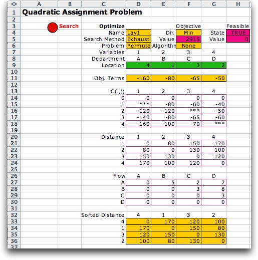
Assignment Costs |
| |
Say the shop owners offer different
rent payments for the locations and some locations are not
suitable for certain shops. These features are added by clicking Include
Assignment Cost box.

|
| |
Another matrix is included on
the form called C(i,j). This gives the cost for making specific
assignments. Here we enter the rent offers as negative numbers.
Since the QAP objective is trip-feet per week, we are subtracting
from that term the revenue per week from rents. It is not really
correct to combine terms with different dimensions. Essentially
we are equating the cost of 1000 trip-feet to 1$ in rent.
The cells with *** indicate assignments that are not allowed.
Although the initial solution uses disallowed assignments,
the search processes will not allow them. |
| |
|
| |
The solution process
enumerates all possible permutations that do not use the disallowed
assignments and returns the optimum.

|
|
Eliminating the restricted
assignments, the location problem now has only 11 feasible
solutions. The solutions sorted by objective function value
are shown at the left. |
|
Larger Problems |
| |
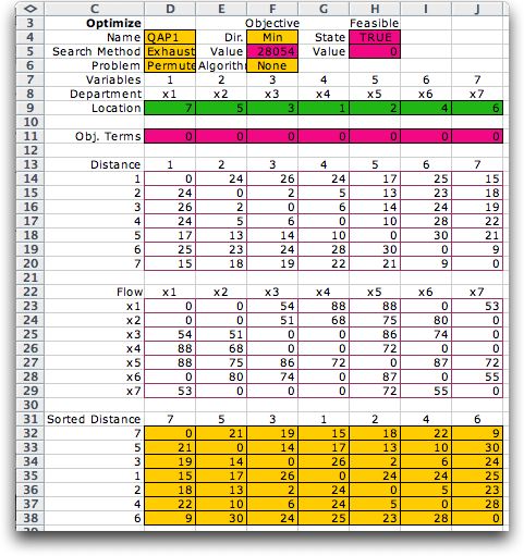
A second example involves six departments
and randomly generated data. The solution of the model found
with exhaustive enumeration is shown in row 9.

|
| |
Exhaustive enumeration requires 5040
function evaluations. The top 20 solutions are listed below.
Since the evaluations use Excel functions, the time required
is a modest 19 seconds on the author's computer. |
| |
|
| |
We add the assignment cost feature
to the problem above and indicate that 50% of the assignments
are to be disallowed. Since a random generation procedure is
used, the fraction of disallowed cells will be only approximately
50%. |
| |
|
| |
The add-in estimates that 2250 solutions
will be enumerated, but there are only 189 feasible permutations.
The estimation procedure is not very accurate when some of the
assignments are disallowed. |
| |
|
| |
The figure below shows the sorted
solutions for a problem with 12 departments. The number of permutations
is far too large for exhaustive enumeration. Alternatively, we
have randomly generated 100 permutations and subjected each to
a 2-change improvement process. The results required over 25,000
objective function evaluations and 164 seconds. There is no way
to tell if the best solution found is the optimum. |
|
| |
The add-in places no limitation on
the size of the problem that can be modeled except the limits
imposed by the size of the Excel worksheet and whatever limits
Excel may impose on the number of functions that may placed on
a worksheet. Of course larger problems are hard to solve. Certainly
exhaustive enumeration is impossible for problems with more than
10 departments unless the allowed assignments are highly restricted.
The greedy enumeration method of the Optimize add-in does not
work for this problem, but random generation is certainly possible.
The n-change improvement option can be applied to the randomly
generated solutions, and given sufficient time, one should be
be able to find good solutions to practical problems. |
| |
|
|
|


