|
|
 |
Combinatorics |
 |
-
Path Tree |
|
For the shortest path tree
problem, each arc is assigned a length. Given a spanning
tree, the distance from the root node to a specified node
is the sum of the lengths for the arcs on the path to that
node. The goal is to select a spanning tree so that the
tree determines a shortest path to every node. This is
called the shortest path tree problem.
To create an instance of the problem we choose Path
Tree from the Combinatorics menu. The Optimize add-in
performs some of the operations used by the Combinatorics add-in,
so both must be installed to formulate and solve problems.
|
|
|
Enter the name and number of nodes
in the boxes provided and select the goal of maximizing or minimizing.
The section at the bottom specifies whether random data should
be provided and the characteristics of the data. The example for
this page is symmetric. |
|
| |
The add-in creates a new worksheet
and places the combinatorial form in upper left corner as shown
below. The worksheet is given the name of the problem and a
number of ranges are also labeled with the name as a prefix,
so the problem name cannot be changed once the form is constructed.
|
|
| |
The example is similar
to the one used to illustrate the spanning tree but some of
the arc lengths have been changed to have a more interesting
solution. With randomly constructed problems, the shortest path
tree often connects the root node (1) directly to each node.
This is the default initial solution, so the results are not
interesting. The example has symmetric arc lengths. This is
an important observation since the greedy algorithm provides
the optimum solution when the arc lengths are symmetric.
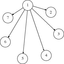
The initial solution shown in row 9 of the worksheet
and illustrated below is constructed with an arc from node 1
to each of the other nodes. The lengths of the selected arcs
are computed with an INDEX function and placed in row 10. Row
11 computes the path length to each of the nodes. For the initial
spanning tree an entry in row 11 is simply the length of a single
arc. For a complicated spanning tree an entry may be sum of
several arc lengths. The objective computed in cell F5 is the
total of all the path lengths or the sum of the numbers in the
colored range of row 11. Minimizing this sum is equivalent to
minimizing the individual path lengths.
|
Greedy Solutions |
| |
The worksheet includes three buttons.
The Search button transfers control to the Search
dialog of the Optimize add-in where all the direct
search procedures are available. The Greedy and Improve
buttons construct additional matrices on the worksheet and perform
algorithms that yield the greedy and improved solutions for
the shortest path tree. Choosing the Greedy button,
presents the dialog below.

Choosing Cancel abandons further processing. Choosing
No initiates the algorithm without a graphical interface
and places the result in the green field of row 9. We choose
Yes to illustrate the instructional features of the
add-in. To perform the greedy procedure, the add-in places a
new matrix on the worksheet below the data matrix called Greedy
Measure. We show the worksheet after several iterations.
The greedy measure is different than the one used for the spanning
tree problem. |
|
| |
The status of the nodes, solved
or not, are shown at the borders of the matrix. The example
above shows that nodes 1, 2, 4, 5 and 6 are solved while 3 and
7 are not. At the left of the measure matrix we see a column
labeled Dual. This column holds the lengths of the paths to
the solved nodes. The numbers correspond to the dual of a linear
programming formulation. The unsolved nodes have the value 0.
The numbers in the dual column are transferred from row 11 where
they are computed. The graph below shows the same information
with the arc lengths adjacent to the arcs and the path lengths
in the brackets adjacent to the nodes.
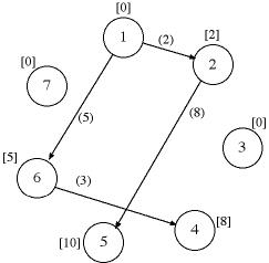
The measure matrix holds large numbers for arcs that are not
candidates to enter the tree, and smaller numbers for the arcs
that can. Specifically, an arc that passes from a solved node
to an unsolved node is a candidate. The measure for the candidate
is the length of the path to its beginning node plus the arc
length. For example, the cell outlined in red representing the
arc from 6 to 7 has the measure:
path length to node 6 + arc (6, 7) length =
5 + 5 = 10.
The add-in uses Dijkstra's
Algorithm for the greedy method. That algorithm adds
the arc that passes from a solved node to an unsolved node with
the smallest measure. We see in the measure matrix that there
are 10 candidates and the one with the smallest measure should
enter the tree. This is the one outlined in red, arc (6, 7).
The figure below shows the final solution obtained after one
more step.
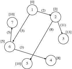
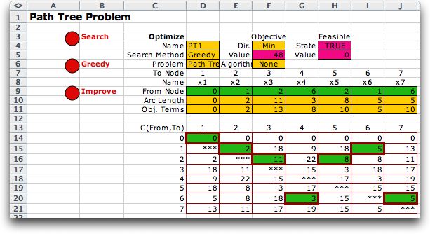
The worksheet with the final solution is shown
below. Dijkstra's algorithm is assured to give the optimum tree
for symmetric networks when all arc lengths are nonnegative. |
Improved Solutions |
| |
To illustrate the improvement procedure
we continue with the same example. Clicking the Improve
button initiates the improvement process. For the shortest path
tree problem, this is equivalent to the primal simplex method
specialized to the shortest path problem. The worksheet below
shows the first and final step for the solution obtained above
with the greedy algorithm. The matrices used for the improvement
process are placed below the data. They look similar to the matrices
used for the greedy algorithm however there are some differences. |
| 
|
| |
There is an entry in the measure
matrix for each arc that indicates the marginal change in the
objective function when that arc enters the spanning tree. For
example if arc (4, 3) enters the solution, the arc that currently
enters node 3 must leave in order to have a spanning tree. That
is arc (2, 3). Considering node 3, the current path to node
3 has a length of 13. If (4, 3) replaced (2, 3) the length of
the path would be increased to 8 + 15 or 23. Then the marginal
change of adding (4, 3) to the tree is 10. Since this number
is positive, the change will increase the objective function.
In general, the marginal change in the objective value when
an arc currently not in the tree is allowed to enter is:
marginal value = path length to the start node
+ length of the arc - path length to the end node
For arc (4, 3) this is
marginal value = path length to node 4+ length
of (4,3) - path length to node 3 = 8 + 15 - 13 = 10
When all the marginal values are positive as in
the example above, the solution must be optimum.
To illustrate a case when the solution is not
optimum we show the worksheet when we try to improve the initial
solution having all nodes connected directly to node 1. |
|
| |
There are several negative entries
in the measure matrix, and any arc associated with a negative
entry could enter to improve the tree . The add-in chooses the
most negative cell and indicates that it should enter. In this
case it is arc (2, 5). When arc (2, 5) enters the tree, arc
(1, 5) must leave. The process continues until there are no
arcs with negative marginal costs.
The improvement process used by the add-in is equivalent to
the primal simplex method applied to the shortest path tree
problem. It will find the optimum for any network, symmetric
or not, as long as there are no cycles with negative length.
For the example, all arc lengths are positive, so the improvement
method results in the optimum solution.
The add-in does not allow an arc to enter the tree if it forms
a cycle. Thus if the add-in is applied to a network with negative
cycles, the add-in will terminate, but the result may not be
the shortest path tree. The search procedures of the Optimize
add-in must then be used to find the optimum.
If we maximize rather than minimize the objective for the model,
the resulting problem is not necessarily optimized by the greedy
or improving methods. The results obtained with the greedy algorithm
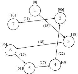
for a maximize objective is the tree shown below. This solution
does not find the longest path to each node, because the collection
of longest paths does not form a tree. For example the longest
path form 1 to 3 is certainly not the single arc from 1 to 3.
The corresponding worksheet is shown below. The
solution cannot be improved with the improvement process. |
|
| |
Solving the problem with exhaustive
search obtains the following best 20 solutions. The optimum has
a total objective value of 366, larger than found by greedy search. |
|
| |
Many of the calculations required by the greedy
and improvement algorithms are done using Excel worksheet functions
in the measure matrix. This is much faster than the enumerative
approach of the Optimize add-in, allowing larger problems
to be solved.
When the model is symmetric and has all nonnegative arc lengths,
the greedy method finds the optimum shortest path tree. With
asymmetric arc lengths or negative arc lengths, but no negative
cycles, the greedy algorithm may not find the optimum tree,
but the improvement process does find the optimum starting from
any valid spanning tree. If the network has negative cycles,
the optimum tree is not assured by either the greedy or improvement
processes.
The model with a maximization objective does not represent
the longest path tree problem. The problem is difficult in that
simple methods do not necessarily find the optimum, rather,
combinatorial search methods are necessary. |
Graphics |
| |
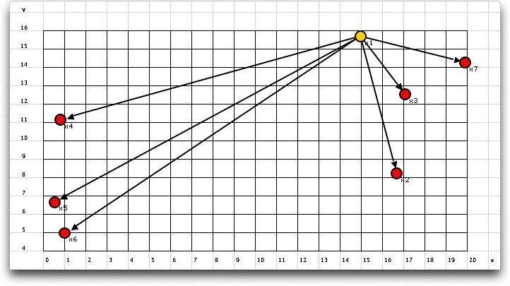
When the arc lengths are computed with a Euclidean
measure, random locations are chosen for the nodes and the distances
are computed. An example is shown below with the optimum already
determined. Not surprisingly the optimum tree has an arc directly
from the root node to each of the other nodes. In Euclidean space,
the shortest route between two points is a straight line. |
|
| |
Clicking the Map button illustrates the
optimum. Where some of the arcs are not allowed (***), the tree
many be more interesting. When distances are truncated to integers,
as in the example, it is possible that the solution to have more
than one arc in a path. |
 |
| 
|
|


