|
This and the next page consider
two combinatorial tree problems that are relatively easy
to solve, the minimal spanning tree problem and the shortest
path tree problem.The Optimize add-in
also considers these problems (spanning
tree and path
tree), but provides more general solution procedures
that evaluate a solution by actually placing the solution
on the worksheet. The Combinatorics add-in requires
that a data matrix specifying the arc lengths be provided.
It uses this distance matrix and Excel computations to
perform the greedy and improvement methods. For some instances
of problems in this class these methods will result in
the optimum solution. For others, the solutions may not
be optimum. The methods of the Optimize add-in
can then be used to search for the optimum.
For the minimal or maximal spanning tree problems, each
arc is assigned a length. The goal of the problem is
to select a spanning tree so that the total of the lengths
of the selected arcs is minimized or maximized. To create
the problem we choose Spanning Tree from the Combinatorics menu.
The figure on the left also shows the Optimize menu.
The Optimize add-in performs some of the operations
used by the Combinatorics add-in, so both must
be installed. |
|
|
Enter the name and number of nodes
in the boxes provided and select the goal of maximizing or minimizing.
The section at the bottom specify whether random data should be
provided and the characteristics of the data. |
|
| |
The add-in creates a new worksheet
and places the combinatorial form in upper left corner as shown
below. The worksheet is given the name of the problem and a
number of ranges are also labeled with the name as a prefix,
so the problem name cannot be changed once the form is constructed.
|
|
| |
The example has symmetric arc lengths
with the length from node i to node j equal
to the length from j to i. . The variables
in the green field (row 9) describe the initial tree. The value
of a variable tells where the tree arc starts. For example,
the value of x2 equal to 1 means that arc (1, 2) is
part of the tree. Node 1 always has x1 = 0. This means
that the tree is rooted at node 1. The initial tree has a total
arc length equal to 96. Although the Feasibility cells
(H4 and H5) are included in the form, they play no role for
the tree problems.

|
Greedy Solutions |
| |
The worksheet includes three buttons.
The Search button transfers control to the Search
dialog of the Optimize add-in where all the direct
search procedures are available. The Greedy and Improve
buttons construct additional matrices on the worksheet and perform
algorithms that yield the greedy and improved solutions for
the problem. Clicking the Greedy button, presents the
dialog below.

Choosing Cancel abandons further processing. Choosing
No initiates the algorithm without a graphical interface
and places the result in the green field of row 9. We choose
Yes to illustrate the instructional features of the
add-in. The add-in places a new matrix on the worksheet below
the data matrix called Greedy Measure.This matrix is
created even if the graphical interface is not used, but it
is deleted after the process. The user should leave the region
immediately below the problem data empty of data or formulas. |
|
| |
The status of each node, solved
or not, is shown at the borders of the matrix. The example above
shows that node 1 is solved and the others are not. The add-in
uses Prim's
Algorithm. The algorithm adds the arc that passes from
a solved node to an unsolved node with the smallest length.
For the first step, only node 1 is solved, so only the arcs
leaving node 1 are candidates to enter the tree. In the columns
immediately to the right we see the minimum length and the node
number that obtains the minimum. The first step must add the
arc from 1 to 4 to the tree.
The figure below shows the next step. The cell
(1, 4) is colored and outlined in the length matrix and the
next arc (1, 7) is outlined in the measure matrix. |
| |
| |
The process continues
until the final solution is obtained. The measure matrix is
deleted upon completion.

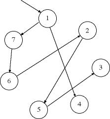
The variables describe the tree below, which is
the minimal spanning tree rooted at node 1.

For symmetric lengths, Prim's algorithm finds the optimum for
the minimal spanning tree problem, so there is no point on going
further on this example.
The measure matrix performs most of the steps of Prim's
Algorithm. It is entirely implemented using Excel functions,
so all necessary computations are extremely rapid. The complete
result is obtained in a much smaller time than when using the
methods of the Optimize add-in, allowing larger problem
instances to be solved in reasonable time. |
Improved Solutions |
| |
To illustrate the improvement procedure
we show a second example with non-symmetric arc lengths. The worksheet
with the greedy solution is shown. With non-symmetric arc lengths
Prim's algorithm does not necessarily obtain the optimum. |
| 
|
| |
Clicking on the Improve button
provides the opportunity to observe the algorithm. The figure
below shows the first and also the last display for the process
applied to the example. The add-in has placed the Improvement
Measure matrix below the data. A cell of this matrix holds
the difference between the length of an arc and the length of
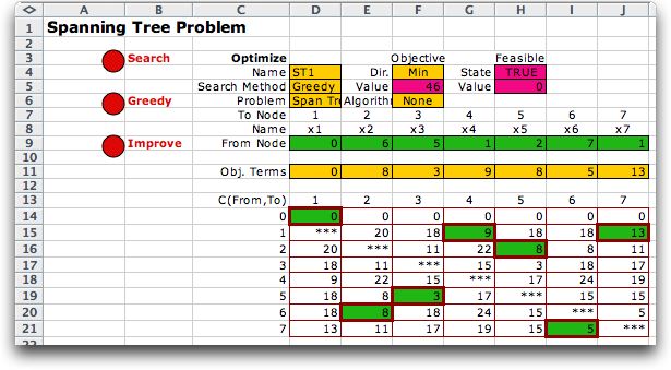
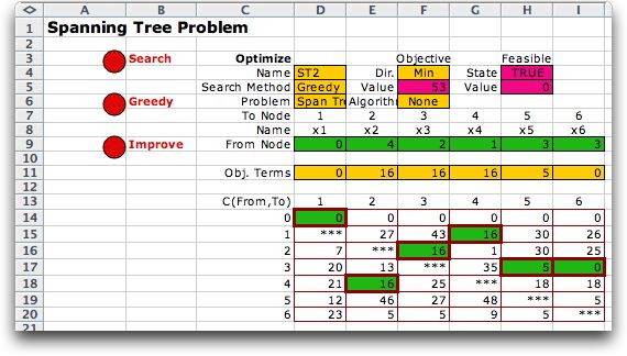
the current tree arc entering a node. For instance, we see that
arc (4, 2) with length 16 is part of the tree, while arc (6, 2)
with length 5 is not. The measure for arc (6, 2) is 5 - 16 = -11.
The negative sign indicates that if arc (4, 2) were deleted and
arc (6, 2) were added, the objective would decrease by 11. We
do not take this step because the result would be a cycle (6,
2), (2, 3), (3, 6). Since cycles cannot be part of a tree we cannot
make this improvement. The improvement step evaluates all negative
numbers in the measure matrix and chooses the one that results
in the most improvement without creating a cycle. It happens that
several entries in the measure matrix are negative, but all form
cycles with the current solution, so the improvement process terminates. |
|
| |
The improvement approach does not
guarantee an optimum. We start with the arbitrary solution shown
below. In the first step, the improvement process suggests arc
(6, 3) will reduce the objective by 38. |
|
| |
The next step finds that arc (3, 5)
can replace arc (1, 5) without forming a cycle and result in a
savings of 25. |
|
| |
The process continues for several
steps until the final solution is obtained. This happens to be
the optimal directed spanning tree. |
|
| |
Many of the calculations required by the improvement
algorithm are done using Excel worksheet functions in the measure
matrix. This is much faster than the enumerative approach of
the Optimize add-in, allowing larger problems to be
solved.
For symmetric networks, the greedy algorithm obtains the optimum.
For asymmetric the greedy method may fail to find the optimum,
and the improvement algorithm also may fail.
The add-in also solves the maximum spanning tree problem. Again
the greedy algorithm finds the optimum for symmetric networks,
while for asymmetric networks, there is no guarantee of optimality. |
Graphics |
| |
When distances are determined with a Euclidean
measure, the add-in offers the opportunity to graphically display
a solution. The arc lengths below are computed using the x
and y coordinates in columns K and L. The lengths are
truncated to integers. A new button, Map, is available. |
|
| |
The example is solved with the greedy method. Since
all distances are positive and the matrix is symmetric, we know
that this is the optimal spanning tree. Clicking the Map
button causes a new worksheet to be produced with a map of the
optimal solution. The gold colored node is the root node. |
|
| |
A more interesting map is the minimal spanning
tree solution of the 48 city problem att48. The data for this
problem represents the 48 state capitals of the continental United
States. The TSP solution is on another page
of this section. |
|
| |
|


