|
|
 |
Combinatorics |
 |
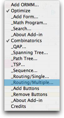
-Routing
Problem - Multiple Vehicles |
|
The Routing/Multiple command creates
a model that is the same as the Routing/Single command
except that more than one vehicle (called trucks in
the following) can serve the sites of the problem. The more general
class of problems is called the Vehicle Routing Problem (VRP).
This model can address a variety of practical situations. |
|
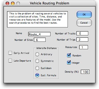
The dialog has
the same features as the single vehicle case except three
new fields are provided. The Number of Trucks field
indicates the number of trucks that can be sent on independent
routes at the same time. The Number of Trips field
indicates the number of separate trips these trucks can
take. A number greater than the number of trucks indicates
that a truck can take more than one trip in a day, but
must visit the depot between each trip. A Resource is
some feature of a truck that is used up when the truck
visits a site. The program allows more than one resource.
The minimum number is 1.
|
|
| |
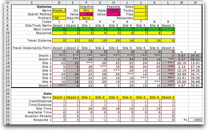
Features of the problem are illustrated
by the example. It is the same as used on for the single vehicle
problem except here there are two trucks serving the six
sites. The two trucks are identified by the headings Depot
1 and Depot 2 in columns D and E of the model. The data in
these columns refers to the two trucks. Column L has a third
depot entry, Depot 3. This column represents the end of the
route.
The distance matrix starts in row 15. A single depot is assumed
and the distances related to all depot columns (D, E and L)
are the same. We color these entries gray to show that they
are determined by formulas and should not be changed directly.
The location of the depot in the x, y columns (columns
M and N) controls all the distances related to the depot columns.
The initial decisions in row 9 define a route that visits
each site in numerical order. Since the first two indices represent
separate trucks, the solution does not have interest. It will
be changed when we search for the optimum. |
| |
|
| |
One new data item appears below
the distance table and that is row 33 holding the resource
values. The resource is something that is provided by the truck
but is used up by the sites on its route. Resources could represent
weight, deliveries, packages or some other measure of capacity.
Here we use the site count as capacity and indicate that each
truck can visit half of the sites. Each truck has a capacity
of 3 and each site reduces this capacity by 1 (the resource
contribution of a site is -1). The number labeled P1, the value
1000 in cell M33, is the penalty for violating the resource
constraint.
Computations related to the resource are in rows 44 and 45.
Row 44 computes the cumulative resource use of the route. Whenever
a depot (or truck) is encountered on the route, the resource
of the truck is placed in the associated cell. For the example,
truck 1 in column D contributes the resource value of 3 in
D44. Since the route immediately passes through the depot,
truck 2 contributes its resource value of 3 in E44. The resources
contributed by trucks do not add as it is assumed that every
time the route passes through the depot a new trip begins.
As the route proceeds through the sites, the cumulative value
of the resource declines until it becomes negative. Columns
I though K show negative values in row 44. A negative value
indicates a shortage of the resource. Shortages are reported
in row 45. The total cost of shortage is the total shortage
multiplied by the shortage penalty. It is computed in cell
N45. All these quantities are automatically computed with Excel
formulas indicated by the yellow color of the cells. |
| |
|
| |
The travel, duration and shortage
costs are added in cell F5 at the top of the worksheet. This
is quantity is the objective function that is to be minimized. |
Optimization |
| |
We choose a solution method by clicking the
Search button on the worksheet. The button calls a
dialog from the Optimize add-in for selecting the
solution method. The dialog shows the Random search
method chosen. This means that 10 random solutions will be
generated and the best of the ten solutions will be reported.
We did not choose the Exhaustive option in this case
because it requires over 5000 solution evaluations.

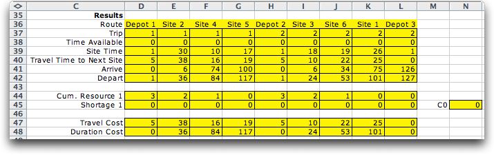
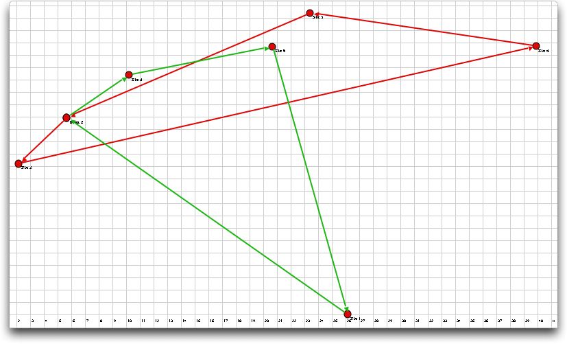
The results of the random search are shown below. The route
follows (Depot 1, 2, 4, 5, Depot 2, 3, 6, 1, Depot 3). This
solution implies that truck 1 serves sites 2, 4 and 5, and
truck 2 serves sites 3, 6 and 1. Notice that the arrival and
departure times indicate that the two trucks operate at the
same time, both starting at time 0. The solution has no shortage
since each truck serves three sites. The total cost is 555. |
| |
|
| |
The map showing the route is below. The route
has two parts the first truck is shown in red and the
second in green. |
|
| |
To improve the solution, we again click the Search button,
but then choose to improve the current solution.

|
| |
The resultant solution is shown below. The
route follows (Depot 1, 6, 5, 4, Depot 2, 3, 2, 1, Depot 3).
The total cost of this solution is 513.
The map for this solution is below. |
|
| |
Additional investigation
may find better solutions. |
|
| |
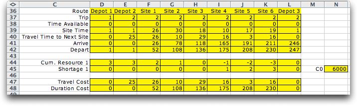
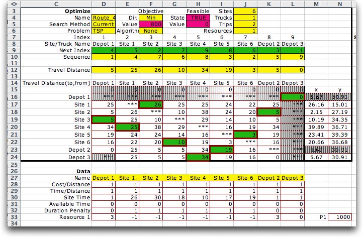
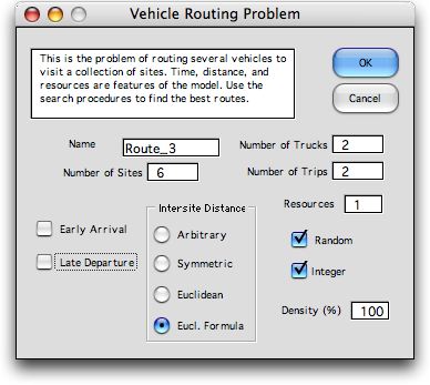
With more trips than trucks, a truck
may cover more than one trip. The trips occur sequentially in
time. To illustrate, consider a problem with a single truck,
but with two trips.
The model shows one depot column (column
D) at the left of the form, representing a single truck. Two
depot columns are at the right (columns K and L). Column K
describes the second trip of the truck, while column L is the
destination at the end of the route. The resource row (row
33) assigns 3 to each truck and -1 to each site. The solution
shown in the figure is the result of the search process described
below. |
|
| |
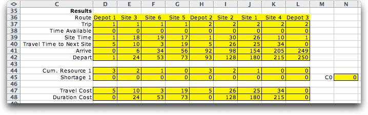
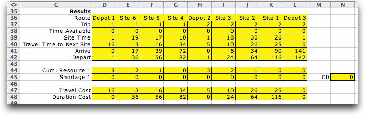
We search for the optimum by first
generating 10 random solutions and then improving the best
of these. The results are shown below. The
route follows (Depot 1, 3, 6, 5, Depot 2, 2, 1, 4, Depot 3).
The total cost of this solution is 800. The interesting part
of these results is the row labeled Arrive. Although
the solution includes two trips, they are both accomplished
by a single truck. After leaving site 5 at time 73. The truck
arrives at the depot at time 92. One minute later it leaves
for the second trip. The truck returns to the depot after the
entire route is complete at time 249. |
| |
|
| |
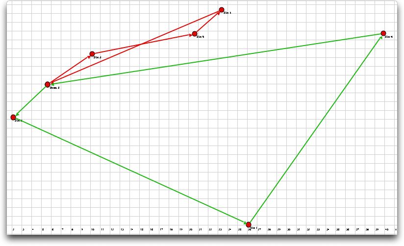
The map describing the solution
is below. Notice the first trip indicated by the red lines
is much shorter than the second trip. This is due in part to
the duration penalty. The penalty causes sites with high site
time and located far from the depot to be serviced as late
as possible.
|
|
|
| |
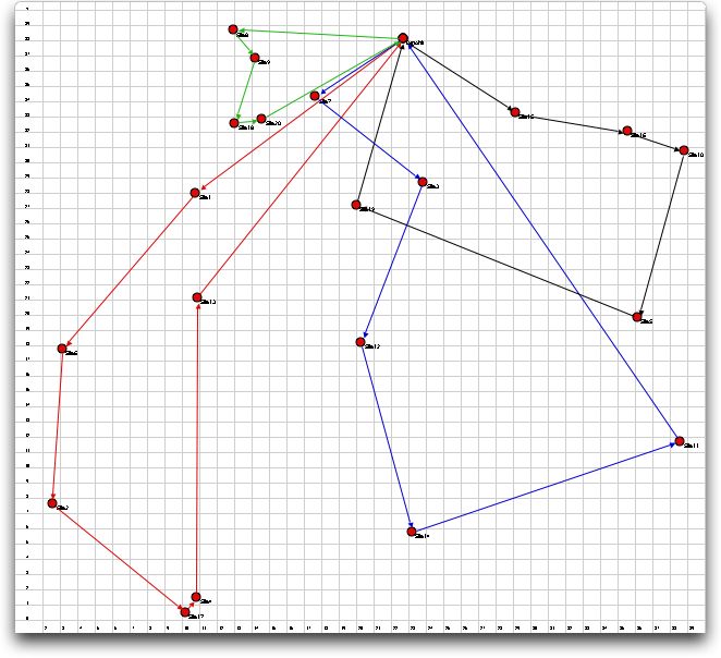
The previous examples used multiple trips because
of limited resources. Time windows also create the necessity
for extra trucks and multiple trips. To illustrate, I created
a problem with 20 sites, two trucks and four trips. Each trip
is given a resource of 5, so that a feasible solution
divides the sites evenly between them. Each site was given
a latest departure time of 240 minutes. Although
the problem is too large to present here, it is included in
the demonstration file for this section. A solution was found
by choosing the best of 100 randomly generated solutions. The
2-change improvement method was applied to that solution. A
map of the solution is below. |
|
| |
The red and green trips are for the first truck
and the black and blue are for the second. The solution shown
is not feasible because the first trip has six sites. A feasible
solution obviously exists, but the search did not discover
one. The solution also has some late departures. |
| |
|
|