An illustration for simple recourse comes from a 1956 article by Allen R. Ferguson and George B. Dantzig, The Allocation of Aircraft to Routes - An Example of Linear Programming under Uncertain Demand, Management Science, Vol. 2, pp 45-73 (1956). The numbers in this example come from the original article and the description was adapted from the Roger Wetts book.

Deterministic Equivalent

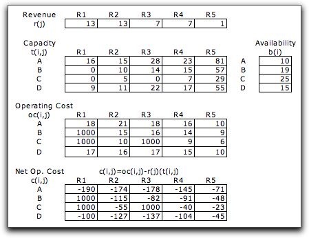
An airline has four aircraft types (A, B, C, D) that fly five routes (R1, ..., R5). Data regarding the aircraft and passengers are given below. The figure comes from an Excel worksheet used to solve the problem. The data reflects 1956 prices and is scaled. The data here is linked to data items on the math programming model, so a different instance can easily be constructed and solved. Revenue gives the revenue per passenger on each route. Capacity is the number of passengers per aircraft for each aircraft-route pair. Operating Cost is the cost of operating a single aircraft on a route. The Net Operating Cost is the cost of operating the aircraft less the revenue for a full aircraft. We express this as a negative number because we will be minimizing the objective. Availability gives the maximum number of each aircraft type to be scheduled. Some aircraft cannot be used on some routes as indicated in the tables as zero capacity and high operating cost.

Our goal is to find the number of aircraft to send on each route to minimize the total net operating cost. If the number of passengers willing to travel on each route were known we could write this problem as a linear program. We write the demand constraints as "<=" because it may not be optimal to satisfy all the demand. The negative values of the objective coefficients encourage the demand to be met, but the aircraft availabilities and capacities may make that impossible.

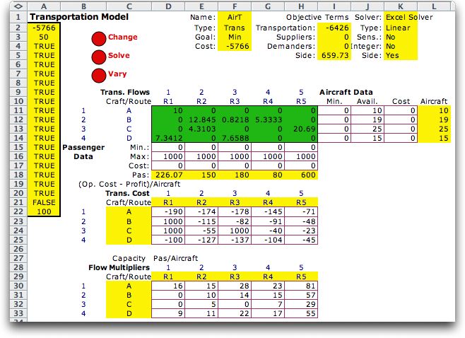
This model has the form of a generalized transportation problem because the variables are multiplied by non-unit coefficients in the demand constraints. The transportation model feature of the Math Programming add-in allows this variation by including flow multipliers. The figure below shows the model with the data of this instance. The aircraft capacities are reflected in the Flow Multiplier matrix. The demands used in the figure are the expected passenger demands computed from the probability distributions given later.

The figure shows the optimum solution with the expected demands. The solution does not meet all the demand for route 5. Indeed there is no feasible solution that meets all the expected demand.

Recourse Model

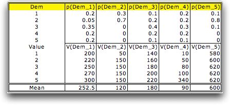
The deterministic solutions do not recognize the uncertainty in demand. The demand for the routes are independent random variables with the values and probabilities shown in the table below. The table was constructed with the Add Random Variable command from the Random Variables add-in. The case shown is an indexed distribution. There is a column for each route with Dem_k indicating the demand for route k. The probabilities are given at the top of the form and the values of the discrete random variables on the lower part of the form. For example, route 1 has demand of 200 with probability 0.2.

When considering randomness, the aircraft allocation problem is a simple recourse model. We must choose the allocation of aircraft to routes before the demand is known. After the demand is realized we find there is either a shortage of demand (assigned capacity exceeds demand) or an overage of demand (demand exceeds assigned capacity). In case of overage, the aircraft flies fully loaded and there is no penalty since the original objective coefficients were computed assuming full use of capacity. When there is a shortage, the aircraft flies with empty seats. 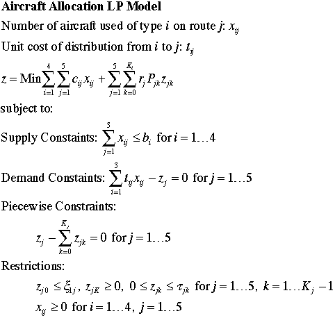The unit penalty assigned is the revenue not received. The simple recourse model is below. The z variables compute the total capacities allocated to the routes. We use general notation to allow any number of points in the distribution, but for the example, there are five possible demands for each route.

For convenience we have computed the cumulative distribution and the step intervals below. We have also created the transpose of the two matrices because the data is used in the model in the transpose form.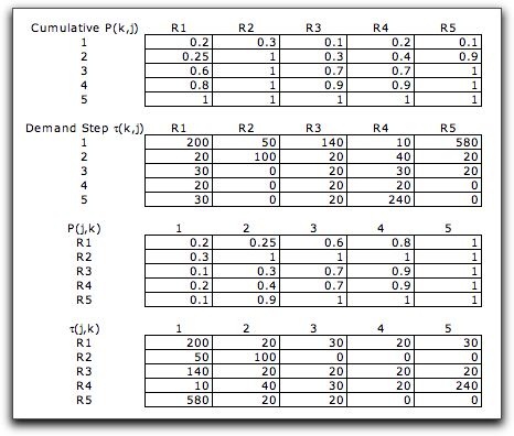

To solve this problem, we create a master problem and subproblems. The master problem has the same format as considered earlier except we do not restrict the maximum passenger flow (row 16). The solution shown is optimum for the master problem when the side problem constraints and variables are included. The "Yes" in K5 indicates that the side problem is to be included in the optimization.

The submodels of the side problem are presented in two parts below. For a side problem linked to a transportation form, the references to the linking variables require two indices. These references are on rows 42 and 43 in columns T through X. Since the transportation variables are arranged in an array, each linking variable is referred to by row and column indices, rather than by a single index as with an LP or network model. The linking variables in this case are the total seats allocated to each route. These numbers are in row 18 of the master problem. For purposes of the indices the transportation flow matrix is extended to include the flow received row (row 18 above) and the flow shipped column (column L). The index for the flow received row is 8. The relevant cells represent the seats allocated are (8,1), (8,2),...,(8,5).

The variables in columns Z through AE are the parts of the piecewise linear representation of the expected recourse cost. The parameters for these variables are in the second part of the side model display. The upper bounds are the demand steps and the objective coefficients are the cumulative probabilities. The shortage costs for the routes are the weights in column R.

The recourse model can be solved for integer flows by simply requesting that the variables be integer through the Change button at the top of the master problem. Results are compiled below for the solutions without and with integer restrictions. The expected value solutions, on the left, restrict the demand met by the allocation to the expected value of demand. The recourse solutions, on the right, recognize the uncertainty of demand through the recourse costs and optimize the net profit with an allowance for demand shortages. Quite different solutions are obtained. Since we are minimizing, the expected value solutions have better (more negative) net costs. This is because they assume all seats allocated are used. In fact, seats may be empty so not all revenue will be realized.

Models representing uncertainty are not too large with simple recourse. The example above could have been easily adjusted for more complex probability distributions. The methods of the Approximation page could have been used for demands with continuous distributions.

This problem is most readily modeled using the transportation format of the Math Programming add-in. The side model feature is adaptable to this structure. With a side model, the problem is actually solved as an LP by the Excel Solver. The free version of the Solver can handle only 200 variables, so the number of master and subproblem variables cannot exceed that amount. The side model grows only linearly with the number of random demands, so quite large models can be constructed on an Excel worksheet. The ability to solve these models depends on the capacity of the Solver.

The Jensen Network Solver does not have the ability to solve models with side problems.