One way to find a solution that explicitly represents uncertainty is to use chance constraints. Again we use the deterministic solution as a starting point. On a previous page, we discovered that the solution below is not satisfactory if the RHS values are random variables. When the RHS values vary about the mean values according to a Normal distribution with a standard deviation of 10, the solution is feasible only about 5% of the time. One way to find a solution that has a greater feasibility probability is to make the RHS vector smaller. All random variables considered on this page are statistically independent.

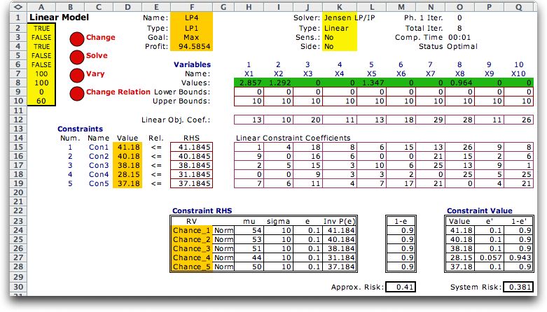
One way to provide values for the RHS with known risks of infeasibility is to use the Inverse Probability function of the Random Variables add-in. The worksheet below shows our LP model and also five probability distributions created by the random variables add-in. The random variables are defined in the outlined range starting in row 23. The parameters of the distributions are in columns H and I. We have placed the desired risk of 10% in column J. Column K holds the inverse probability values. For example, there is a 10% chance that the RHS for constraint 1 will fall below 41.1845. This number is computed in cell K24 with the expression:

=RV_inverse(Chance_1,J24)

The number is transferred to the LP model with a formula in cell F15:

=K24

In the figure below, each RHS is set to a value so that there is only a 10% probability of violating each constraint individually. This is easily accomplished by setting the values in the range J24:J29 to 0.1. The deterministic solution shown is optimal for the RHS values shown. The objective value is 94.6. This is quite a bit less than the value of the expected value solution, 125.5, but this solution has a much greater probability of feasibility.

Although the probability of violating each constraint is only 10%, the probability of violating at least one of the six constraints is considerably greater. An estimate of this probability is:

The system risk is computed in cell M30 of the worksheet. The estimate is an upper bound because some constraints may not be tight at the optimum solution, for example, constraint 4 is loose. The estimate for the risk is 0.41 for the present case.

A better measure of system risk is computed at the right bottom of the figure. Here the constraint values obtained by the solution are used to compute the probability that the constraint limits will fall below the values obtained by the solution. The probabilities for the individual constraints are computed as e'. Assuming independence the system risk of 0.381 is computed with the expression.

Levels of Risk

Different solutions may be obtained with different levels of risk. Several solutions are presented below with increasing objective values and increasing risk. The constraint risk is the number used to determine the RHS values, and the system risk is the probability that the solution will violate at least one constraint. Any number of solutions could added by selecting different values of risk for the several constraints.

In this example, the RHS values are independent random variables and we have included chance constraints for each individual constraint. Since the analyst is probably interested in finding a solution with a given system risk, it would be useful to construct a single constraint that assures this result. This is called a joint chance constraint. Unfortunately, this constraint is not easy to write. For simple cases, it may be possible to write the constraint, but the resultant model is not a linear program. In fact, the feasible region of the resultant model is probably not convex, making the model difficult to solve.

Even if we use only individual chance constraints, there is no general guidance on how to set the risks of constraint violation. The chance constraints do give the analyst a method for explicitly recognizing uncertainty.

Different Forms

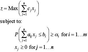
The mathematical model of an LP with chance constraints can be written as below.

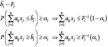
As noted above the probability statement can be replaced with a linear constraint with the RHS replaced a constraint evaluated by the inverse probability function. A different form is required for a ">=" constraint. For an equality constraint there is no chance that the constraint will be satisfied for any given solution. So the risk is always 100% for an equality constraint for continuous probability distributions.

We have considered on this page only randomness for the RHS values. When constraint coefficients are random, the situation is more complex.