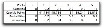
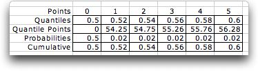
To approximate the continuous distribution we select K+1 quantile values ranging from 0 to 1.

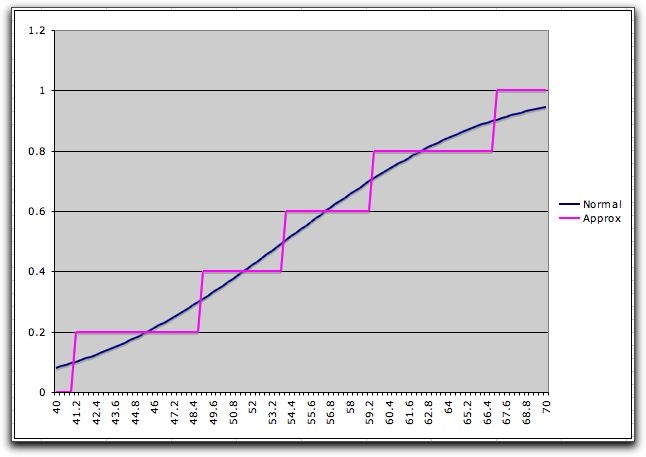
To illustrate, consider a Normal distribution with mean 54 and standard deviation 10. We divide the probability range into five intervals using the quantiles: 0, 0.2, 0.4, 0.6, 0.8, 1. The quantile points are computed with the RV_Inverse function of the Random Variables add-in.

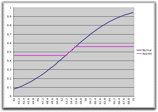
The graph below shows the cumulative distribution of this discrete approximation (in magenta) along with the Normal distribution (in blue). The picture shows the steps as ramps, but the steps are perpendicular at the quantile points. The approximation sometimes over estimates the continuous cumulative and sometimes underestimates it.

The number of steps and the selection of the quantiles controls the accuracy of the approximation.

Simple Recourse

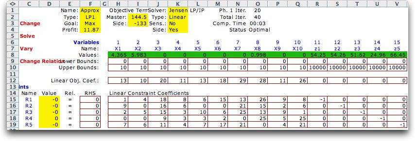
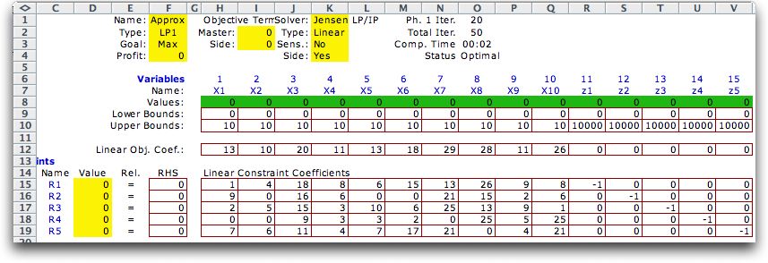
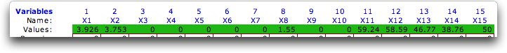
We return to the ten product mix problem considered earlier, but now we will solve it as a simple-recourse model. The master problem below includes the production variables and the variables computing the resource usage.

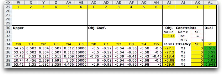
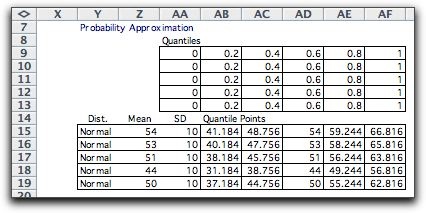
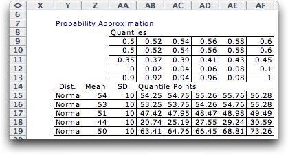
To the right of the model we have constructed tables to compute the necessary probabilities and quantile points from the quantile values specified by the modeler. Normal distributions are defined in columns Y through AA. All computations relating to these distributions are provided by functions in the Random Variables add-in. Other distributions could just have well been used.

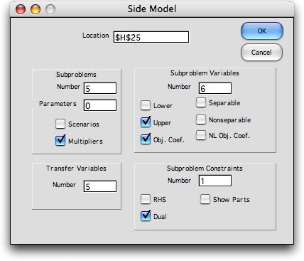
The piecewise linear representation of the expected recourse costs are expressed in the side model. Build the side model by choosing Side Model from the Math Programming menu. Fill in the dialog as below.

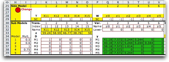
The model is constructed starting in cell H25. We show the model in two parts below. The first part identifies the linking variables through the indices in row 30. Columns J through O provide information on T and D. The variables and the associated W matrix are in columns P through V. For definitions of the matrix terms, see the side model discussion. The multipliers in column I represent indicate the penalties associated with the violating the resource constraints. For this discussion we charge $1 for each unit of resource shortage and $0 for each unit of resource overage.

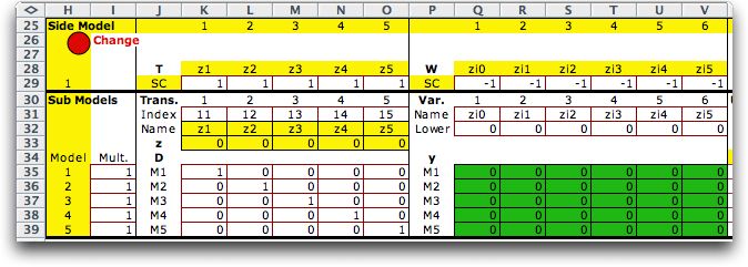
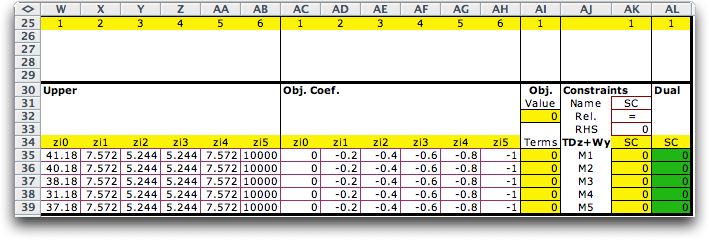
The upper bounds defining the piecewise approximation are in columns W through AB. The associated objective coefficients are in AC through AH. The numbers in these cells are linked by formulas to the table constructed for the piecewise linear approximation. For details, see the demonstration workbook for this section.

The constraints in AK require the equality between the linking variables and the pieces. The relation and limit of the side constraints are in cells AK32 and AK33 respectively.

Solution

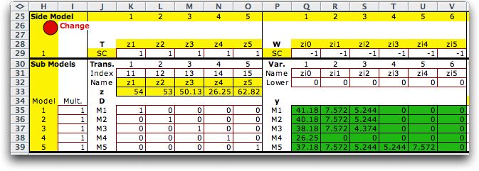
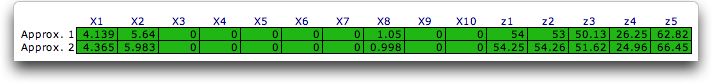
Clicking the Solve button at the top of the page provides the solution shown below. The resource usage variables, z1 through z5, are in both the master and subproblems. The production variables are x1 through x8. The green cells in the side model show the results for the pieces of the piecewise linear form.

The important point of this discussion is that simple recourse is relatively easy to model and solve with linear programming. The individual stochastic part of the problem is modeled with a deterministic equivalent. The expected cost of the resources are piecewise approximations of the continuous expected cost function.

More accuracy may be obtained by adding more pieces to the approximation or more accurately representing the expected value in the region of the optimum. The search is aided by the dual variables of the side constraints shown in column AL of the figure above. This approach is considered below.

A Better Approximation

The solution obtained above provides information about the optimum use of the resources of the product mix problem. In particular the dual variables shown in column AL show the probabilities that the resources will be violated at the optimum solution. The first resource, represented by the first side constraint, has a dual variable of 0.561. Solution uses 54 units of R1 and the mean availability of R1 is 54 so really the risk of violating the resource is 0.5. Our piecewise approximation causes the error of 0.061.

We obtain a more accurate approximation by defining quantile points that emphasize the probability range 0.5 through 0.6.

The cumulative distribution shown below is more accurately represented in this range, while it is not well approximated outside the range. This feature will have usefulness for the simple recourse model.

Based on the solution found with the rough approximations for the Normal distributions, we modify the quantiles under consideration to cover a smaller range of probabilities. In the table below we define five intervals in a 0.1 range for each random variable.

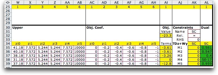
The optimum solution is shown below for the revised quantiles. The value of the expected recourse cost is quite distorted by the approximation, so the optimum objective function is markedly different for this solution. The approximation adds a negative constant to all solutions, so the decision values obtained are the optimum for the more accurate representation. The slopes of the terms of the objective function of the LP determine the optimal solution, and the slopes in the smaller range are much more accurate than with the first approximation.

The dual solution provides an interesting interpretation. The dual indicates the risk that each constraint will be violated when the optimum solution is pursued. Clearly the last constraint, indicated by M5, is the most important constraint. The solution will have a shortage with respect to this RHS in over 95% of the future realizations. Apparently, the profit obtained by using more of this resource is sufficient to pay for the cost of its violation. Of course the optimum solution and the risks depend on the penalties.

The two solutions are compared in the table.

Different Penalties