|
|
 |
Stochastic
Programming |
 |
-
Wait and See |
|
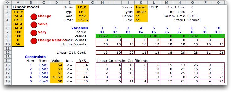
To illustrate stochastic programming,
consider the linear programming model below. The solution algorithm
is the Jensen LP/IP add-in. The problem was generated randomly
using the Math Programming add-in. The solution shown is the
optimum solution when all parameters of the model are deterministic. |
|
| |
For the examples on this page, we assume that
all parameters are deterministic except the right-hand-side
vector,
shown in the range F15:F19. The numbers given are the expected
values but we add a random variation for each value that is
distributed
as a Normal variant with mean 0 and a standard deviation of
10.
On this page we investigate the wait-and-see policy
in that the random variables are realized before the decision
maker sets
the solution vector x. The solution x is
determined by the solution of the LP. This is not really a stochastic
programming problem because there is no uncertainty when the
decisions are finally made. We might be interested, however,
in the stochastic features of the optimum solution value
and on the feasibility of the model when viewed before the
random variables are realized. On this page we use the Monte
Carlo simulation features of the Random Variables add-in
to perform the analysis. |
The Stochastic Model |
| |
The methods of this section are
applied to an optimization model constructed with the math
programming add-in. We have created the LP model above on the
worksheet LP1.
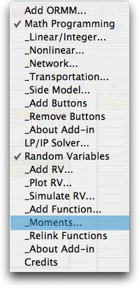
To create a stochastic model that describes the random features
of the situation, we choose Function
from the Random Variables
menu and fill in the Add Function dialog as below.
We have specified LP/IP as the algorithm in the field at the
bottom
of the dialog.
This means that the LP will be solved
for each point of the sample space that is generated by the
enumeration or simulation procedure. For the example we use
the Simulate method. |
|
| |
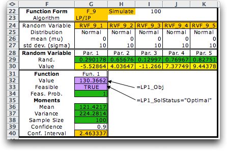
The form is placed below the LP model as shown
below. The information in rows 22 and 23 give the function
name, F_9, the type of analysis, Simulate, the number
of simulation iterations, 100, and the algorithm to be used
with each iteration, LP/IP.
The random variable definitions
are in rows 25 through 27. All
have
been specified
as Normal
distributions
with
mean values of 0 and standard deviations of 10. The parameters
can be changed on the form. The math programming model
is linked to the random variables via the RHS entries shown
in column F of the LP model. They have been replaced by the
equations in column G (the equations are placed in column
F, but illustrated
in
G). Each RHS is the sum of the original value stored in column
C and a Normal random variable defined on the function form.
As the simulation is performed the RHS values will change
randomly.
|
| 
|
| |
Rows 28 through 30
generate the simulated values. The numbers in row 29 (now 0.5)
will be replaced by uniformly distributed random numbers. The
numbers in row 30 compute the simulated values based on the
Monte Carlo method.
Rows 31, 32 and 33 describe the functions to be
observed during the simulation. Cell G31 is the name. The function
value in G32 is an equation that links to the LP objective
in F4. The feasibility value in G33 is
a logical statement that points to cell O4 (shown with the
LP model above). That cell, filled by the LP/IP add-in, holds
the word "Optimal" only when the model has a feasible
solution. For each simulation these cells will hold the optimum
LP value and an indication of feasibility. The particular solution
shown has all random variables set to 0,
their expected
values.
The
solution
for
this sample
point is the same as the deterministic solution.
The green cells in the range G34 through G38 hold
the results of the simulation. These are filled in by the add-in.
Cell 34 returns the proportion of the observations that are
feasible. Cells G36 and G37 hold the mean and variance of the
simulated function, the LP optimum value in this case. Only
the results for feasible solutions are reported. Cell G38 holds
the number of feasible solutions or the sample size of the
mean and variance statistics immediately above. G39 holds a
confidence level entered by the user, cell G40 holds a confidence
interval computed from the statistics.
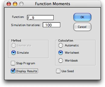
To simulate the model choose Moments from
the Random Variables menu and set the number of simulation
observations to 100. Larger values give more accurate results,
but take
more
time. Each simulation iteration draws a random sample from
each distribution. The
values are
reflected
in
the RHS
vector,
and the LP/IP algorithm
solves the problem. |
|
| |
The results of
100 observations are combined and placed on the form beginning
in row 34 of the figure below. The numbers shown in rows 29 through
33 are for the final simulated observation of the random variables. |
| |
|
| |
We have simulated 100
observations of the wait-and-see option. Even though
the solution is optimum for each simulated RHS, the mean objective
function
(estimated at 121.4217 in cell G36) is lower than the value
when the RHS values were set to the expected values (125.6).
This is a consequence of "Jensen's Inequality" (named
after a different person than the author). The expected value
solution
will always have a higher objective function (when maximizing)
than a solution that explicitly represents uncertainty.
All the observations in the sample of 100 were
feasible for the example and the 90% confidence interval for
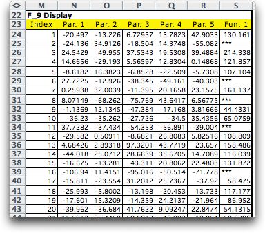
the LP objective value is almost 2.5. The
add-in displays the random variable values as well as the objective
function values. The first 20 observations are shown below.
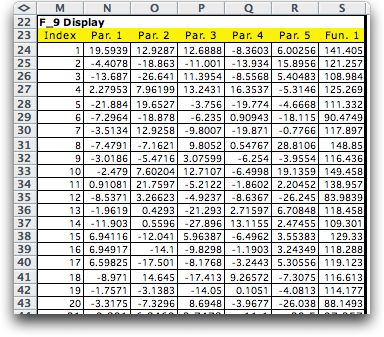
It is interesting to increase the standard
deviation of the random variables to 30, thus increasing
the variability of the RHS values. The simulated results are
below.
For this model, the solution is infeasible only if one of
the RHS values is negative. With the data provided, 77% of
the right side values have feasible solutions. The mean objective
value is decreased with significantly greater variance over
the case when the standard deviation values were 10. The 90%
confidence interval is now about 8.25. There is a price to
pay for variability, even with the wait and see policy. |
| |

|
| |
For the example
shown in the figure, the value of the random deviation for the
fifth constraint is -68.427. This is larger in magnitude than
the mean value of 50. The negative RHS value allows no feasible
solution. The list below shows the first 20 simulated values.
The *** values in column S indicate that there are no feasible
solutions for the associated simulated values. |
| |
|
| |
On the next and
following pages, we consider the problem of setting the variables before the
random variables are known. |
| |
|
|