|
|
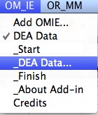
With installation
of the DEA add-in, the
menu for the add-in is added to the OM_IE menu. The figure to
the left shows the DEA menu. The Mathematical
Programming and LP/IP add-ins on the OR_MM collection should
also be installed. The Mathematical Programming add-in constructs
the LP models used for the analysis. The LP/IP Solver solves
the model. Alternatively the Excel Solver can also be used
to find solutions. Read the section for the Mathematical
Programming add-in for more details. The DEA add-in requires no user interaction
with the Math Programming or LP/IP add-ins.
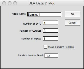
The DEA Data item from the menu presents the DEA
Dialog shown on the right. The dialog accepts a problem
name. This name is used for range names on the model worksheet
and also the worksheet name, so it must contain no spaces
or punctuation. The name should not be changed manually after
the model is built. Try to make the name short.
The problem parameters are numbers of DMU's, output factors
and input factors. The Beasley problem has four DMU's, two output
factors and one input factor. These numbers can be changed after
the model has been created. Checking the Make Random Problem checkbox
causes random data to be placed on the model form. This is handy
for demonstrating the add-in features. The Random Number
Seed initiates the built-in random number generator for
Excel, so the data depends on the random number seed. The data
is not entirely random as there is some correlation between input
and output factors. |
| |
|
|
| |
The Start command
on the DEA menu should be used after opening a DEA data file
the first time. This command replaces all the buttons on the
worksheet pages. If you download the DEA Demo file, you must
run the Start command
to control the program. The Finish command deletes all
the buttons from a worksheet. It is good practice to run the Finish command
if you plan to open the file on a computer different than the
one that created it. |
The Data |
| |
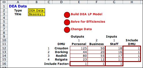
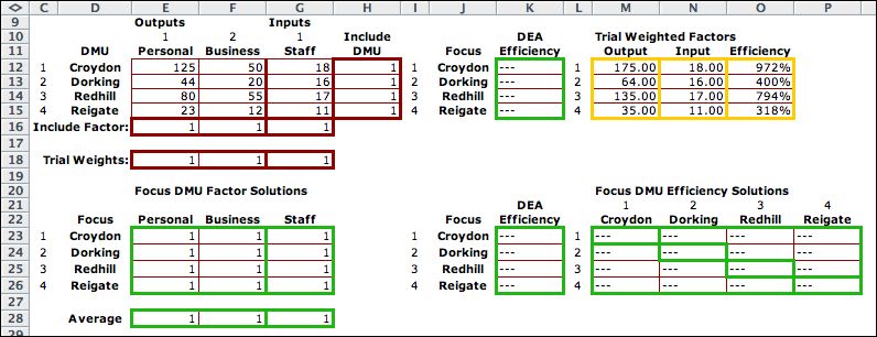
A new worksheet is
created in the current workbook.The figure shows the upper-left
corner. DMU, Output and Input Titles that
head the rows and columns of the data array may be changed.
The output-input data fills the cells of the table. Control
buttons are above the data items.
The Include DMU column
is provided to add or remove DMU's from the analysis. If the
include input is 0 for some DMU, the data for that DMU does
not affect the analysis. The value 1 includes
the DMU. Similarly the Include Factor row allows for
inclusion or exclusion of a factor from the analysis. Of course
there must always be at least one input and one output factor
included. The include options are often useful for a practical
analysis. The include elements must be 0 or 1. The maroon outlines
for the data indicate that these are to be filled by the user. |
| |
|
Weights for the Factors |
| |
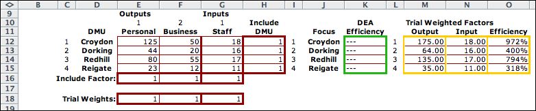
Below the data region
is a vector for trial weights. To the immediate right is the
DEA Efficiency for the DMU's. Computed cells are outlined in
green. The analysis places numbers in this range. To the right
we see the weighted outputs and inputs. The output values
in column M and the input values in column N
are computed using the SumProduct
function with
the trial
weights,
the include data and the the factor data.
The efficiency values of column O divide the weighted
output with the weighted input. The yellow
outlines indicate that the cells are computed with formulas.
Initially the weights are all 1, so the output column is the
sum of the outputs and the input column is the sum of the inputs.
The efficiency values are well over 100%, so these weights
are not valid. |
| |
|
The Results Matrices |
| |
Again we expand our view
of the worksheet to show the matrices where DEA solutions are
stored. The DEA solution process solves a series of LP models.
Each model finds the optimum weights for one DMU. When all the
DMU's are included there are four LP problems solved. The DMU
index defining the LP model is called the Focus. The
solutions for the four focus DMU's are placed in the rows of
the results matrix. |
| |
|
The Solution |
| |
The Solve
for Efficiencies button at the top of the page constructs
the LP Model and solves it for each focus DMU. The LP solution
variables are shown in the Focus DMU Factor Solutions matrix.
The Croydon solution weighs the personal
transactions output, but gives 0 weight to business
transactions.The other solutions use nonzero weights for
both factors. |
| |
|
| |
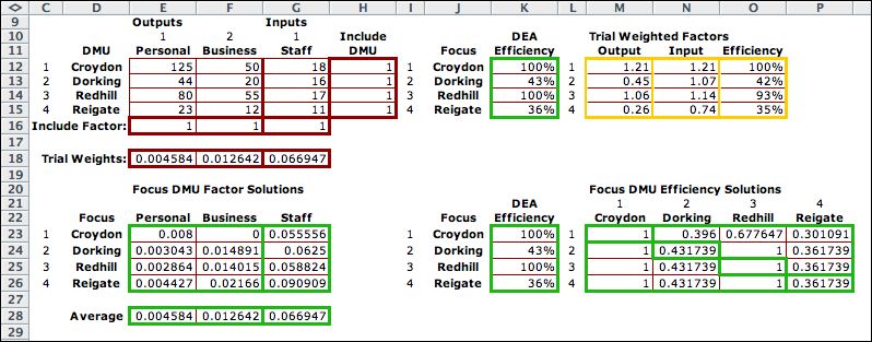
After each LP solution
the program places the values of the optimum weights in the trial
weights row. The formulas in column O compute the corresponding
efficiency values. The transpose of these values are pasted
in the Focus DMU Efficiency Solutions matrix. The
DEA efficiencies are found on the main diagonal of the matrix.
The DEA efficiencies values are outlined in green in column
K.
The range in row 28 called Average is the average
of the weights for all the included DMU's. At the end of the
process these weights are used for the Trial Weights.
The resultant efficiency values in column O shows the relative
efficiencies of all four DMU's for this weight selection. This
result can be used to rank the DMU's. This may not be a good
practice, however, since the solutions may be degenerate. The
DEA method was not designed to obtain a complete ranking, rather
a relative ranking that identifies the undominated DMU's with
DEA efficiency 1. DEA efficiencies less than one identify dominated
DMU's.
Croydon and Redhill both have DEA efficiencies of 1 and Dorking
and Reigate have lower DEA efficiencies.
The next page discusses the LP model. It is not necessary
for the user to deal with the LP model directly. Its setup
and solution are controlled by the add-in. |
The LP Model |
| |
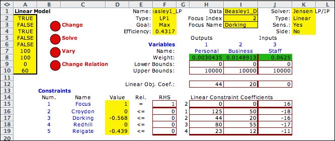
Clicking the Build
DEA LP Model button at the top of the page calls the Math
Programming Models add-in to construct the general LP
model
for the focus DMU. The model for Dorking is shown below. All
the model coefficients are filled by formulas linking to the Data
page.
The Focus Index in cell I2 specializes the model to
the focus DMU. The coefficients in the objective function and
the first constraints are the output values and input values
for the focus DMU. This number can be changed manually to see
how the model is constructed, but it is automatically varied
by the solution algorithm. The other constraints are the same
for each DMU. |
| |
|
| |
The buttons in column
B can be used to change features of the solution process as indicated
in the Math Programming Models add-in documentation.
Clicking the Solve button solves the LP model for the
focus DMU.
Clicking the Solve for Efficiencies button creates
the LP if it does not exist. It then solves the LP model for
each included DMU and transfers the result to the data worksheet.
The LP model is on a separate worksheet that the data, so it
need not be addressed directly. Model building and solving
are automatically performed by the add-in when the buttons
on the data worksheet are clicked.
The next page of this discussion describes the LP model in
more detail. |
| |
|
|