Clicking the top button on the DEA data sheet calls the MP Models add-in to build the appropriate Linear Programming (LP) model. The data is transferred to the LP model with equations that point to the input, output and DMU data on the data worksheet. Clicking the second button uses either the Jensen LP/IP solver or the Excel Solver add-in to solve the sequence of LP models to fill the DEA Efficiencies and the other results matrices on the data worksheet.

It is not necessary to click the first button to prepare for the solution. Rather, simply click on the second button. If the LP is not already present in the workbook, it will be constructed before proceeding with the DEA solution steps.

The LP Model worksheet

The LP model focusing on the first DMU, Croydon, is shown below. All the data on this worksheet is linked to the numbers on the data worksheet. It is unnecessary to enter any data yourself, unless you have defined extra variables or constraints. The model shown below has already been solved. The index of the focus DMU is in I2 and its name is in I3. The columns of the LP present the output and input factors as specified on the data worksheet.

The objective of the LP model is to maximize the DEA efficiency of the focus DMU. The variables are the factor weights in row 8. Variables are required to be nonnegative using the lower bounds on row 9. Upper bounds in row 10 are set to be non-binding. The first two objective function coefficients in row 12 are the unit output values. The columns for inputs have 0's in the objective function.

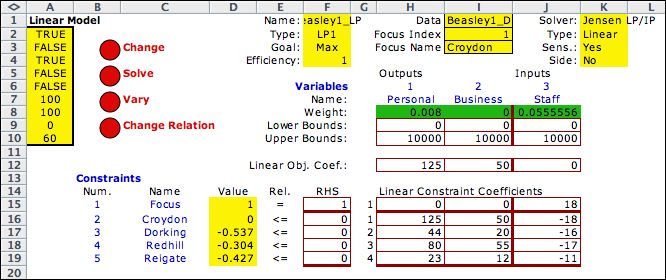
The first constraint in row 15 requires the total of the weighted input values to be 1. The coefficients of the first constraint for the outputs are 0, while the unit input values for the focus DMU are in the input columns. (18 in this case). This constraint is an equality as indicated by the "=" in E15. The remaining constraints are derived from the efficiency limitations that require the ratio between inputs and outputs be less than or equal to 1.

The buttons on the LP model worksheet control the Math Programming add-in. They can be used to add constraints or variables to the model. Clicking the Solve button solves the current model. For Croydon, the solution determines the weights that maximize the efficiency for Croydon. The objective value in F4 is the DEA efficiency.

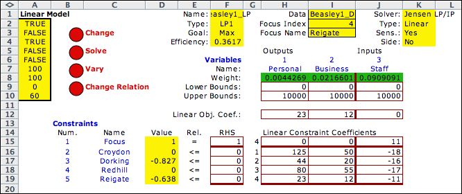
The LP model for Reigate is shown below. To get a new focus DMU simply enter its index in I2. The coefficients of the objective function and first constraint change, but all other LP data remains the same.

The Complete Solution

When the Solve for Efficient Solutions button is clicked, the add-in sequentially solves the LP for each DMU. The LP solutions are copied from the variable values on LP model and pasted in the appropriate row of the Focus DMU Factor Solutions table. As each solution is obtained it is also pasted into the Trial Weights range. The values of formulas in the Efficiency factors in column O are pasted into the corresponding rows of the Focus DMU Efficiency Solutions. The DEA efficiencies are on the main diagonal of this table.

Finally the range labeled Average in row 28 is transferred to the Trial Weights range. This gives the complete ranking of DMU's in column O. This ranking should be taken with caution however since they can be manipulated by using alternative optimum solutions as the factor solutions.

Changing the Models