Computation Section
Subunit Data Envelopment Analysis (DEA)
 - Manager's Response

Each branch manager returns to his or her branch and pledges to compute the efficiency measure to his or her advantage. Recall the data for the branches and the subsequent analysis used by the executive.

beasley data

Adding the two output measures together provides a single measure of output. When divided by the staff number, the ratio is the number of transactions per staff member. When the ratios are normalized the results are called efficiencies. The best efficiency is recorded for the Croydon branch and the other branches are ranked below Croydon. To quell arguments the CFO, agrees to allow the managers to select their weights independently. Adding the two output measures together is equivalent to proposing equal weights for the factors.


The Croydon Branch


Jane, the branch manager of the Croydon branch, meets with her assistant and relates the meeting with the bank CFO. The assistant points out there is no point in further calculations. Croydon already has an efficiency of 1 using equal weights, and additional analysis cannot yield a better result. Jane proposes the weights of 1/(175+18) for the two outputs and 1/18 for the staff. She is sure that she will win.


The Dorking Branch


Joe, the branch manager 
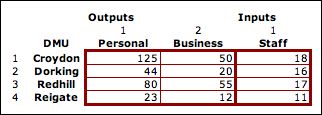
of the Dorking branch does not have it so easy. His branch has fewer transactions in both categories as Croydon. The branch does have a smaller staff than Croydon. Perhaps if he gives a larger weight to staff and less to the transaction outputs, he will get a better efficiency. Joe had an OR course in college and knows that OR has methods for optimization. He finds his old textbook and looks up the term optimization. He learns that he needs to have an algebraic mathematical model.

His job is to select the weights, so he defines variables for the output and input factors.

branch notation

The efficiency for Dorking is the ratio of the weighted outputs over the weighted input. We index the branches in the order they appear in the data so Dorking has index 2.

Dorking Efficiency

From the formula Joe can see that he can make the efficiency as large as he wants by increasing the output weights and decreasing the input weights. He notes however that the efficiency cannot be greater than 1, so he forms a constraint on the variables.

dorking efficiency sonstraint

Although the ratio limits the variables, they still are unconstrained from above because as long as the output weights are proportional to the input weights, the ratio remains the same. This problem is resolved when Joe sets the weighted input to 1 and maximizes the weighted output.

dorking objective

After some thought Joe realizes that he can not make his decision with data regarding only Dorking, He must assure that the weights assigned do not cause the other branches to have efficiencies greater than 1 or less than 0. The lower bound is easy to assure since all inputs and outputs have positive values. He restricts the weights to nonnegative values. The efficiencies of the other branches are computed with similar formulas since all branches must use the same factor weights. Unfortunately the ratios are nonlinear and Joe never studied beyond linear programming (LP). For the LP model all the expressions must be linear. It happens that the expressions can be made linear by multiplying both sides of the inequality by the expression in the denominator. The last step in the sequence below moves the variable term on the right to the left side of the inequality. This is the standard form of an LP constraint.

croydon constraint

The complete linear programming model for the Dorking weight selection problem has three variables and five constraints.

Dorking LP

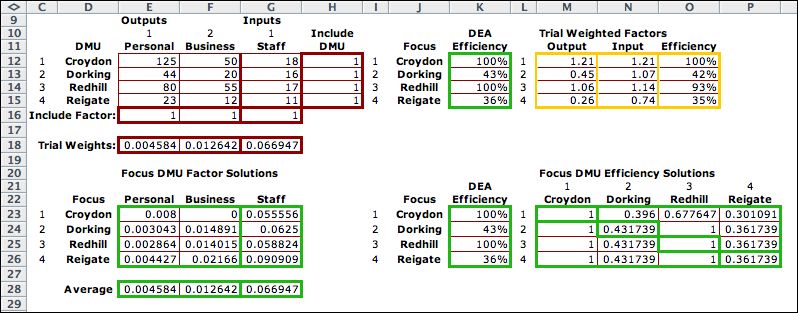
Using the Math Programming add-in the model can be built on an Excel worksheet and solved with the Jensen LP/IP Solver. The figure shows the LP model for Dorking. The LP Solution is shown below in the green field. The objective value is in cell F4.

Dorking LP Solution

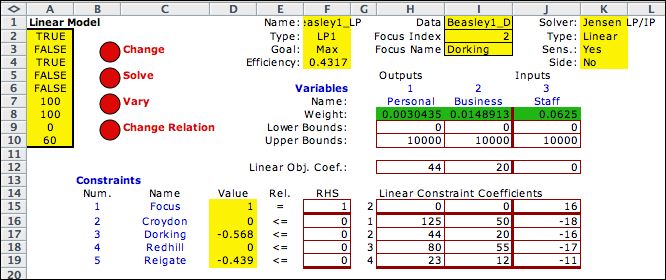
Joe is not happy with the results. The maximum efficiency that Dorking can obtain is 0.4317. The factor weights that solve the LP provide that efficiency, but no other feasible weights will have a greater efficiency.


Every Branch

  Every branch has the same LP model except the objective function and the first constraint. We call k the index of the focus DMU. The figure below lists the notation that specifies the variables and coefficients of the general model.
 
  There is a model separate model for each DMU. The model for DMU k, is shown below. The objective function coefficients are the observed output values for the focus DMU. The first constraint assures that the weighted sum of the input values is equal to 1. Its coefficients are the observed input values. The remaining constraints are the same for all DMU's. They assure that the efficiency ratios do not exceed 1. The non-negativity constraints for the weights complete the model. The analysis assumes all observed output and observed input values are non-negative.
 
general LP


Solution


The clever branch bank managers figure out that the answer to their individual weighting problems are all answered by optimizing the variables in an LP. The four LP's are similar except the objective value and the first constraint. Each is solved independently of the rest. The bank CFO was really asking a question with a preordained answer. She could have answered the question without asking the branch managers.

The figure below, created by the add-in, shows the optimum values for all branches. Each row of the green outlined region starting with row 23 describes the solution of a separate LP. Row 23 begins with the optimum factor weights for the Croydon branch (0.008, 0,0.055556). The corresponding objective value is shown as 100% in the DEA Efficiency column. The matrix starting at M displays the ordinal efficiencies computed with the trial weights in row 18. In this figure the trial weights are the average of the optimum factor weights of the four branches.

Rows 24, 25, and 26 provide the solutions for Dorking, Redhill, and Reigate respectively. Croydon and Redhill have DEA efficiencies of 1 and Dorking and Reigate have lower DEA efficiencies.

Note that the Croydon solution is different than the one shown in the Beasley notes, (0.00271, 0.012642, 0.05556). The DEA efficiency for both solutions is 1. The two answers are both optimum solutions. Beasley's solution was obtained with the Excel Solver with starting values of (1, 1, 1). The solution in the table was found with the Jensen LP/IP Solver with a starting solution of (0, 0, 0). Changing the starting point for both solvers gives the alternative result. Multiple optimum solutions are due to degeneracy in the LP.

 
beasley solution
  We leave the interpretation of these results to the CFO. The literature on DEA has considerable discussion on the interpretation of DEA results, but we do attempt to write them here because of the author's inexperience with the subject. With this add-in I am providing a tool for computing the DEA results. The details of building and solving a model start on the next page.
  
Return to Top

tree roots

Operations Management / Industrial Engineering
Internet
by Paul A. Jensen
Copyright 2004 - All rights reserved