|
|
 |
Process
Flow Models |
 |
- Resources
|
| |
Resources
are used to manufacture products. A resource is characterized
by time available during some interval of time, say 40 hours
per week. Production during the week uses up the time available
for resources, but the resources remain for the next week.
Resources include machines, space and labor. In the context
of an application a variety of resources might be defined.
The economic analysis allows specification of resource investment
costs, operating costs, number and availability. A variety
of questions might be answered for which resources play an
important role.
|
| |
|
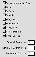
Checking the Resource box
in the dialog causes the process definition to include
resource columns, one for name and another for amount.
The resources described by these columns are called System
Resources and are usually physical resources, such
as machines, that are located in specific places in the
plant. The other boxes checked in the figure, add other
features specific to the example.
The field labeled General Resources specifies
the number of columns to include for resources that are
used for several operations in the process. These usually
are resources that do not involve physical location.
We use labor as a general resource for the example.
Although we do not specify that parameter columns be included,
two columns are automatically created because they are
necessary for the time functions. |
|
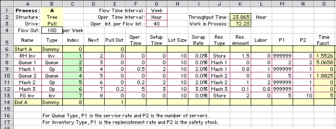
To illustrate we use a serial
pull process with inventories and queues. The triangle
for operation 1 represents the raw material inventory.
The triangle for operation 7 represents the finished
goods inventory. The d-shaped symbols for operations
2 and 4 are delays for the queues waiting for machining
operations 3 and 5.
We add a second pull location at
the output of operation 6. The value of 0.2 indicates
that for each unit leaving operation 7, 0.2 will leave
at operation 6. The two pull amounts are not independent,
the flow withdrawn from 6 will always be 20% of the amount
withdrawn from 7. If independent demands at the two locations
were required, separate processes would be defined for
each pull location.
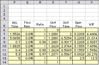
Parameters for the operations are
on the Excel worksheet below. The worksheet is shown
in two parts for clarity. All operations use lot sizes
of 10. Only operations 3, 5 and 6 have nonzero operation
times. Nonzero scrap rates are at the three processing
operations, so their ratios are less than 1, and the
unit flows increase as we move backwards from operation
7. Defects are not included in the model, so there is
no need for inspection. Operation 6 models a batch process
where 10 items are processed at the same time. Each item
passing through the operation has a processing time of
5 hours, but all items in the batch of 10 are processed
at the same time, rather than sequentially. We model
the batch process by assigning 1/10 to the resource amount
for items passing through the machine 3. The denominator
is the batch size.
The process uses resources as listed
in column J. The names of the resources are important,
because the use of like-named resources by separate operations
and separate processes are combined. The names of resources
that appear in column J are also used to construct the from-to matrix.
The four system resources for the example are: store,
machine 1, machine 2 and machine 3.
The entries in column J are called System
Resources. Column K shows the number of units
of each resource used by the operation. The dimension
of capacity may differ between resources. In the example,
the dimension of the store resource is square
meter-hours, while the dimensions of the other three
system resources are machine-hours. The RM Inventory
operation (row 7), uses 1.5 square meters (col. K)
for each unit of flow passing through the operation.
The time required is 1.5526 hours (col. P). Thus each
unit of demand uses 1.5*1.5526 = 2 sq. meter-hour (col.
T) of the store resource. The numbers in column
T are used in the Economic Analysis part of
the model. Machine resources are measured in machine-hours.
We note that the resource use for operation 6 is 0.1,
indicating that 10 units, the size of the batch, will
use up the entire capacity of machine 3.
Labor is a general resource and
its use is described in column L. The three processing
operations require 1, 2 and 0.8 units of labor during
the operation time. The total use of labor per unit of
finished good, leaving operation 7 is determined in the
economic analysis. |
|
| |
|
| |
Data Items for the Example (related
to resources)
Column |
Title |
Explanation |
J |
Resource Type |
This is the resource used by the
operation. Resources are identified with names. Different
operations and processes may use the same resource. The
resource types defined in this column are system resources and
are used for the economic analysis and also to construct
the from-to matrix.
|
K |
Resource Amount |
This is the number of resources used
by the operation. For machines it is usually 1, although
it could be less than 1 if the machine is not used during
part of the operation time or the operation is a batch
process. Resource amounts may be 0. The from-to matrix
recognizes flow that passes from one system resource to
another system resource. In the example, we identify the
queues as using the resources of the machines they precede,
but use 0 as the resource amount. This causes the flow
to be passed from the store resource to the machine 1
resource. If the resource type were left blank for the
Queue 1 operation, that flow to machine 1 would be lost.
|
L |
General Resources |
The dialog allows the user to produce columns for general
resources. An example is labor, where each operation may
require a specified number of labor hours per operation hour.
An entire column is provided for each general resource, so
different operations may use the same resource. The name
of a general resource is placed on the top of the column.
A general resource should not use the same name as the names
listed in the Resource Type column. The numbers
in a general resource indicate the amounts of the resource
used by flow passing through the operations.
|
|
Economic
Analysis - Resource Availability and Use |
| |
The Economic Analysis option on the
OM/IE menu produces the Project worksheet. All parts
of the worksheet are constructed by the add-in with default
data in several areas defined for user input. Generally, ranges
with a white background and maroon outlines are for user data,
yellow areas hold Excel formulas and green areas hold the
output of computer computations. The user data for the example
has been entered by the author to illustrate meaningful values.
Several of the ranges on this worksheet refer
to resources. Although, not specifically showing resources,
we include the Product portion of the worksheet
because the product sales per week (cell I3) drives the total
resource requirements. The number is initially taken from
the Flow Out cell (B4) in the process definition,
but can be changed here to investigate the impacts of different
levels of sales. The example has only one process defined,
otherwise there would be multiple lines in the Product
portion. Although we choose to sell (and manufacture)
100 units of product A which is the output of operation 7
in the process, we also produce 20 units at operation 6. The
product is identified by the process name.

Starting at row 8 for the example (row numbers
will be different for other examples), we see the portion
of the worksheet that accepts data and compiles information
from the processes that are defined in the workbook. The current
example only has one process, so all the information comes
from that process (A).

Column E lists the resource names as compiled
by the add-in from the process definitions. Column F shows the
number of each resource used. For the first three resources,
this is the number of machines used. In the case of store,
this is the number of square meters, and for labor it is the
number of workers. Except for machine 1, we have entered values
large enough to provide sufficient resources to manufacture
100 of product A. column G holds the maximum number of the resources
allowed. Here, we use the same as column F, but this column
will provide an upper bound for the mixed integer programming
model that optimizes the number of the resources. Column H implies
that all resources work for 40 hours per week. Column I indicates
the availability of the resources. Values less that 100% indicate
downtime. Column J is provided to limit the utilization of resources.
Although we exclude variability for our model, we recognize
that WIP will explode when resources are used to high utilization
when there is variability present. Here we allow the user to
specify the maximum utilization allowed. Columns F through J
are user data and can be changed to represent the system being
modeled.
Column K is the hours available for each unit
of resource considering the entries in columns H, I and J. Column
L multiplies this by the maximum number of resources. Column
M is the available hours given the number of resources used.
Column N holds the computed amounts of the resources used given
the sales of the product. For a feasible system, the entries
in column M must be no less than the entries in N. Note that
the row for machine 1 shows a slight deficit, indicating that
the 100 units of production for process A is not quite obtainable.
The primary model assumption is that resource
use is proportional to the number of items passing through an
operation and the time required for the operation. This is valid
in many, but not all, contexts. One case in which it is not
valid is for a queue that uses the resource of space. The number
in the queue, the time in the queue and subsequently the space
required is a nonlinear function of flow. |
Resource
Cost |
| |
Starting in row 16 of the Project worksheet, a table
of resource costs is provided.

Again, the resources are listed in column E.
This list is constructed by the add-in. Data is entered in
columns F through G. Column F has the space per resource unit.
Any space measure can be used, but assume the numbers are
in square meters. The first three entries are the space requirements
for each of the machine types. Since the dimension of store
is square meters, the space per unit is 1. We assume
4 square meters are allowed for each worker. Column G is the
operating cost per hour for each resource. This cost is expended
only for time used. Column H shows the investment cost amortized
to the weekly interval of the analysis. These costs are fixed
costs per unit of resource and do not depend on the utilization.
Columns I though J are computed with formulas
based on the number of hours used to manufacturing 100 of
the A product and the number of each resource provided. The
latter was entered in the range F9:F13. The space requirement
might be useful for a plant
layout analysis. The operating and investment costs are
used in the economic analysis. Totals are provided in row
22.
|
Unit
Resource Use |
| |
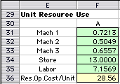
This table starts in row 29 for the example. There will be
as many data columns in the table as there are products, but
here we only have one column. Again the resources are listed
in column E. The green range in the table is computed by the
add-in from the process definitions. Each entry is the amount
of resource used per unit of product. For example, the definition
shows two uses of resource store. The first is the
RM Inventory that for each unit of finished good uses 1.5
meters for 2 hours. The second use of store is the
FG Inventory that for each unit of finished good uses 2 meters
for 5 hours. The total use is then (1.5*2 + 2*5) 13 hours
per unit of finished good A. The Resource Operating Cost/Unit
is the sum-product of the resource operating costs (G17:G21)
and the contents of (F31:F35). This value is subtracted from
the revenue per unit to obtain the operating profit column
of the product portion of the worksheet (cell J3).
|
From-To
Matrix |
| |
A matrix that is useful for plant
layout analysis, is the from-to matrix. The flows
between system resources are computed by the add-in and placed
in the matrix display starting at row 45. The green area indicates
the flows between the system resources listed in column J
of the process definition. Columns and rows are also constructed
for the general resources, Labor for the example.
The default flow in these cells is zero, but if there is a
flow from labor to or from any of the system resources, that
flow can be entered into the cells provided.

|
Summary
and Refilling |
| |
In the upper left corner of the Project worksheet
there is a summary of the economic results. This summary is
linked to the product sales and the results of the various
data items and computations on the worksheet.
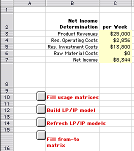
It may be that the user will want to change
process definitions or add new processes. The contents of
the Project worksheet may be updated after changes
by clicking the button to "Fill usage matrices".
The from-to matrix is updated by clicking the "Fill
from-to matrix" button.
|
| |
|
|
