|
|
 |
Process
Flow Models |
 |
- Queues and Inventories
|
 |
There are
features of processes that cannot be modeled by linear models.
This is particularly true of the effects of variability. Although
the process flow model is deterministic and does not explicitly
represent the variability often present, it is possible to include
estimates of the average time delays due to a variety of causes.
We do this by providing an Excel user function call time_f (time
function). Four models are currently built into time_f.
On this page we describe three models: one to model the delays
from queues, another to model the delays due to inventories and
the third to model delays due to changes in lot sizes. A fourth
model that computes lost time due to production lines is on the
next page. |
| |

|
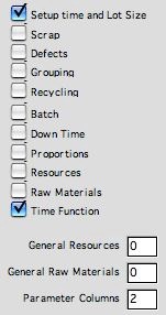
To include inventory
or queue models, check the Time Function box on
the Add Process dialog . It is unnecessary
to check the Setup time and Lot Size box, but
the lot size column is automatically included, whether
or not this box is checked. The lot size column is used
by the time function.
The time function requires two parameter columns. The
user might add other Excel function models in the process
definition. Any number of parameter columns can be included
to hold operation parameters for these models. The number
is specified in the field at the bottom of the dialog. |
|
To illustrate the use of the time
function feature, we use a serial pull process with
inventories and queues. The triangle for operation
1 represents the raw material inventory. The triangle
for operation 6 represents the finished goods inventory.
The d-shaped symbols for operations 2 and 4 are delays
for the queues waiting for machining operations 3 and
5.
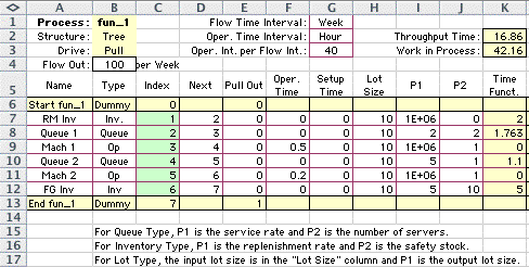
Parameters for the operations are
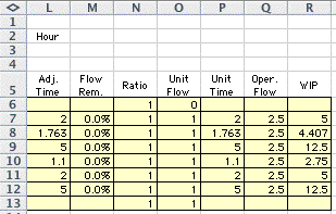
on the Excel worksheet below. The worksheet is shown
in two parts for clarity. All operations use lot sizes
of 10. Only operations 3 and 5 have nonzero operation
times. Scrap and defects are not included, so all ratios
are 1 and all unit flows are 1.
Of interest to the time function
are the two parameter columns, P1 and P2 and the Time
Function column holding the time functions. |
|
| |


|
| |
Data Items and Result Items for the Example
Column |
Title |
Explanation |
B |
Type |
This column is used to identify the
type of the operation. It is particularly important for
the time functions. The time function uses the first three
characters of the type to identify the function to be evaluated, "que" for
queue, and "inv" for inventory, and "lot" for
lot size change. When the type includes the word "line",
the production line formula is
evaluated.
|
H |
Lot Size |
This is the number of units processed
in a lot.
|
I |
P1 |
This is the first parameter column.
The column title may be changed for clarity. For the queue
model, the column holds the average service rate for the
servers of system. For the inventory model, the
column holds the replenishment rate for the inventory system.
The default value, 999999, is meant to represent infinite
service rate or infinite replenishment rate.
|
J
|
P2 |
The second parameter column holds
the number of servers for the queuing model. It holds the
safety stock for the inventory model. Again the title of
the column may be changed. The default value is
1, represents a single server or a safety stock of 1. To
obtain a valid result for a queuing model, the number of
servers must be sufficient to handle the arrival rate.
|
K |
Time
Function |
This column holds the time_f function
provided by the add-in. For the row representing the
raw material inventory (row 7) the function is entered
as below:
=time_f(B7,F7,Q7,H7,I7,J7)
We explain the arguments of the function
for specific applications below.
|
Q |
Operation
Flow |
This is the total flow rate entering
the operation. It is the product of the unit flow and the
process flow V. Both queuing and inventory
models use the total flow rate to compute the operation
delay.
|
|
Queues |
| |
Consider row 8 of the example. It models the
queue for the machining operation described in row 9. The
important information from row 7 is
-
Column B: type = Queue
-
Column H: lot size = 10
-
Column I: service rate = 2/hour
-
Column J: number of servers = 2
-
Column Q: arrival rate = 2.5/hour
The argument in column F is the operation time.
It is not used for the functions on this page.
We have chosen the service rate to be the inverse
of the operation time in cell F9 (1/0.5 = 2). This is reasonable
since the queue is waiting for the service operation in row
9. The minimum number of servers in this case is 2. The result
of the computation, shown in column K, is the average time
each unit remains in the queue. The time does not include
the service time. The service time is added in row 9 that
represents the machining operation that follows the queue.
The queuing model assumes that units are processed
in lots. In general we call Q the lot size. For
the example, Q = 10 units. We assume that lots
arrive according to a Poisson process (the times between
lot arrivals
are exponentially distributed). For the example, the arrival
rate in lots is 2.5/10 or 0.25 per hour. An important result
for an Exponential distribution is that its coefficient of
variation (COV) is 1.
The service time for each unit is exponentially
distributed. The units in a lot are processed individually
and in sequence, so the time to process the lot is the sum
of Q exponentially distributed random variables.
The mean service rate for a lot is the service rate for an
individual unit divided by Q. For the example, this
is 2/10 = 0.2. The sum has a Gamma distribution. An important
result for a Gamma is that its coefficient of variation (COV)
is  . .
We use a non-markov queuing model to compute
the mean time in queue. The formulas used are the same as
used in the Queue add-in. The non-markov model uses
the arrival rate, service rate, number of servers, COV of
the arrival process, and COV of the service process. All parameters
are available from the row for Queue 1.
=time_f(type = "queue",unit arrival
rate,lot size,service rate,number of servers)
The data used for the queuing model is:
The result shown in cell K8 is the mean time
in Queue 1, 1.763 hours. This is actually the queue time
for a lot, but it is also the queue time for each unit. A
unit must wait as long as its lot waits. Holding items in
lots results in significantly increased queue times.
The queue represented in row 10 is similarly
analyzed by the time function to obtain a queue time of 1.1
hours.
|
Inventories |
| |
Inventories are another instance of variability in flow.
An example is the raw material inventory represented for the
example in row 7. Perhaps raw materials must be delivered
by truck and it is more efficient to deliver a quantity (lot)
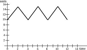
of raw materials than a single unit. Then the pattern of inventory
could be approximated as below.

Using the data for the example, raw materials
arrive in lots of 10 units. Since the flow rate through the
inventory is 2.5 per hour, the orders must arrive every 4
hours. We are assuming here a continuous withdrawal of items
from the inventory, but arrivals occur at discrete times.
The variability causes a delay as units remain in inventory.
The time function that computes this delay has the parameters:
=time_f(type = "inventory",usage
rate,lot size,replenishment rate,safety stock)
In cell K7 we see the function call:
=time_f(B7,Q7,H7,I7,J7)
For the example, the columns holding the parameters
are:
-
Column B: type = Inventory
-
Column H: lot size = 10
-
Column I: replenishment rate = 999999/hour
-
Column J: safety stock = 0
-
Column Q: usage rate = 2.5/hour
The formula for average delay with an infinite replenishment
rate is:

For the example, the average delay for the raw
material inventory is 2 hours.
Row 12 represents the finished goods inventory.
Since that inventory is supplied by Machine 2, we assume that
the inventory is replenished at a finite rate equal to the
inverse of the unit processing time of Machine 2, 5 per hour.
If we assume that product is withdrawn from the system at
a uniform rate of 2.5 per hour, the finished goods inventory
pattern is as below. The inventory variation is on top of
the safety stock. Of course the figure is an abstraction.
Obviously it would be unnecessary to have safety stock in
such a well behaved system. The safety stock is used to handle
the variability of the output demand which in reality is quite
unpredictable.

The time function computes the average time
an item remains in this inventory with the formula below.

In cell K12 we see the function call:
=time_f(B12,Q12,H12,I12,J12)
For the example, the columns holding the parameters
are:
-
Column B: type = Inventory
-
Column H: lot size = 10
-
Column I: replenishment rate = 5/hour
-
Column J: safety stock = 10
-
Column Q: usage rate = 2.5/hour
For the example, the average delay for the raw
material inventory is 5 hours. The safety stock contributes
4 hours, while the cycle inventory contributes 1 hour.
|
Lot Size
Change |
|
|
It is common in some manufacturing systems to have different
operations to use different lot sizes. For example, the
first operation might have a lot size of 1 and a second
operation may have a lot size of 10. Considered in isolation,
we can compute the unit times of the two operations and
use them to compute the throughput time for the system.
This neglects, however, an important interaction that
results in a delay for items passing through the system.
That interaction is the lot size change activity.
When the lot size changes from 1 to 10, there must be
a delay while items from the first operation are gathered
to create a lot of size 10. The WIP created is a function
depends only of the input and output lot sizes. The formulas
are given in the discussion for the Inventory add-in.
The WIP is 4.5 for this example. The time function computes
the appropriate time delay for the lot size change operation.
|
Other
functions |
| |
No doubt there are other features of the process model that
could be implemented as a time function. Other features could
be implemented by changing
the time_f user function. It is accessible through
the Visual Basic code that implements the add-in.
It should be noted that the functions shown in this example
are valid only if the queues and inventories only involve
a single process. If multiple processes share inventories
of raw materials or units from several processes share production
resources, the inventory and queue models should be system
models, and not models relating only to individual processes.
Such system models could be constructed using the data from
the Economic Analysis worksheet. The models could
be constructed automatically, but the current add-in does
not have this capability.
|
| |
|
|


