|
|
 |
Investment
Economics |
 |
-Add
Project
|
 |
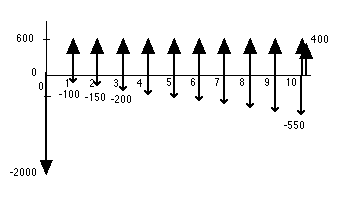
A businessman is considering
the purchase of an asset that has an initial cost of $2000.
The asset promises an annual return of $600. It's operating
cost is $100 the first year, $150 the second, and increases
by $50 in each subsequent year. The salvage value for the asset
in 10 years is $400. The cash flow for this situation showing
the individual components explicitly is shown in the figure
below. If the businessman's minimal acceptable rate of return
is 10%, should he invest in this project?

With the Economics add-in the data describing
the asset is easily entered and a variety of economic analyses
are automatically performed. To enter the data associated with
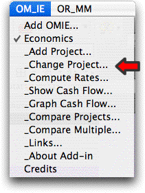
this or any similar situation, we choose the Add Project option
from the menu, |
| |
|
Clicking this option calls a VBA program
that displays the dialog that accepts structural information
about the project as shown below. We see at the top of the dialog
a box holding the address identifying the cell at which the
upper-left corner of the worksheet range where the project information
will be placed. The cell automatically indicates the location
of the cursor when the dialog was called, but it can be changed.
The next box holds the name of the project.
An automatic name is originally presented with the prefix "Proj".
This default name should be changed to some identifying name
related to the situation. We use E6 in the dialog. The name
provided will be part of the Excel names assigned to various
ranges on the worksheet. Once it is assigned it cannot be changed
later. A name is unique to a project in the workbook. It must
obey the naming conventions of Excel. It cannot include spaces
or punctuation other than the underline symbol. |
| |
|
| |
The remaining collections
of boxes and buttons describe features of the cash flow. Two
important quantities are the number of cash flows and the number
of investments. The current example has 5 cash flow components.
We specify the number of investments to be 0, however, we illustrate
an alternative below.
A number of options not used for this example are described
later.
Clicking the OK button, calls a program that constructs the
display below on the worksheet. We show the display with information
already added. |
| |
|
|
| |
Regions
in this display that are colored yellow contain information
or formulas that should not be changed by the student. The
cells are not locked and can indeed be changed, but the worksheet
will not yield correct results. Notice that the name, E6,
is in cell B2. As indicated earlier, this name should not
be changed. Other information from the dialog has been placed
on the display.
In the cash flow data area, five lines
have been constructed to hold data for the example. In the
Description column, we place simple identifiers of the cash
flow components. The Amount column holds the dollar
value of the cash flow item. Here we use negative numbers
(shown in red) for expenditures and positive numbers (shown
in black) for revenues. The Type column is important because
it indicates the type of cash flow. The recognized types
are shown in the table below along with the start, end and
parameter definitions. When interpreting types, the program
only uses the first two letters and ignores case, so "SI" indicates
as single payment as well as "sin".
Type |
Description |
Single |
This is a single payment at a specified time. The value
of the payment is in the Amount column. The time
is indicated in the Start column. The End and Parameter columns
are not used. Examples from the display are the Investment
and Salvage items. |
Uniform |
This is a series of cash flows of uniform values.
The value of each payment is in the Amount column.
The Start column indicates the time of the first
payment and the End column the time of the last.
The two components, Return and Op. Cost, both start at
1 and end at 10. The Parameter column is used
to indicate a uniform series with a cycle time other
than 1. For instance if 2 where entered here, the payments
would be at times 1, 3, 5, 7, 9. The default value is
1 as in the example. |
Gradient |
When the cash flow is a series whose magnitude is increasing
by a fixed amount in each period, the cash flow is called
an arithmetic gradient. The current example is the gradient
in operating cost. The value of the gradient is in the Amount column.
The Start time is the time of the first non-zero
value of the gradient and the End is the time of
the last. The parameter entry describes a cyclic gradient.
The default value of 1 is used in the example |
| Geometric |
This describes a geometric gradient. It is not illustrated
by the example. The first payment is a fixed amount and
each payment following increases by a fixed percentage g from
the previous one:
A, A(1 + g), A(1
+ g)^2, etc.
The value of the first payment is in the Amount column.
The Start time is the time of the first non-zero
value of the gradient and the End is the time
of the last. The parameter in this case is the percentage
growth. The cycle is always 1 for this cash flow component. |
|
| |
The rightmost columns
(H and I) holds computed quantities. The yellow cells (H10:H14)
labeled Factor hold the equivalency factors that convert
the cash flows to equivalent values at time 0, or the present
worth values. These are computed with user-defined functions
that are described on a later page. Cells I10 through I14 hold
the net present worth values for the five cash flow components.
They are computed by multiplying the amounts in column C by
the factors in column I. Since the numbers in columns H and
I are functions, they automatically compute whenever a parameter
changes. The characteristics of the cash flows are parameters
as well as the MARR.
The quantities at the top of the page in column I, hold the
totals for the cash flow. The entry in I2 is the total of the
cash flow component present worth values. I3 is the uniform
equivalent of the present worth spread over the life of the
project. I4 is the present worth over a study period. The study
period used is given in cell D4. It is the product of the life
(D2) and the replications (D3). The study period may be different
than the life when comparing two or more projects. The numbers
in column I are formatted as integer values, however, the number
of decimal values can easily be changed using the Excel formatting
pallet.
For the example, the Present Worth over the life is positive,
indicating that the project returns more than the MARR. The
project is acceptable.
An alternative description of this same example is constructed
with the dialog box below. |
| |
|
| |
Here we specify the number
of cash flows as 3 and the number of investments as 1. The worksheet
representation of the project is below. |
|
| |
Here we see that the
machine investment is described in a separate area called Investment
Data. The investment value is given as the amount and the
salvage value is given as a percentage. The investment takes
place at the start time and the salvage is realized at the end
time. The present worth values of the cash flow are the same
as the other representation. A project requiring several investments
is described by several lines in this investment data area. We
will have special use of this area when considering inflation
and taxes. |
| |
 |
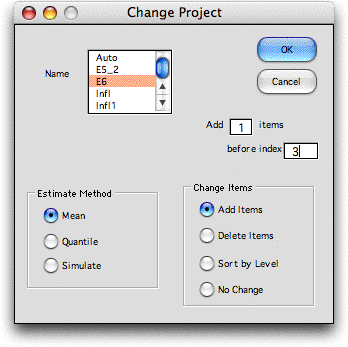
Rows can be added and deleted
in with the Change Project command. On selection,
a dialog is presented as below.

|
|
| |
Select the name of
the project in the Name field. Choose whether to add
or delete items with the buttons at the lower right. The example
would add an additional item to the Project E6. Additions cannot
be made before the first item or after the last. The first
and last item cannot be deleted. The Sort by Level button
does not work at this time. Whenever items are added or deleted,
rows are added or deleted from the project form. Use caution
that the change does not distort other forms on the same worksheet.
The buttons on the left are used for models with probability
distributions representing uncertainty. |
| |
|
|


