-Taxes and Inflation

We consider once more the example, but now we have both taxes and inflation. The combination is interesting because depreciation amounts do not inflate. Inflation discourages large investments, since the positive effects of depreciation are not realized until the years following the investment. As the years go by, the real value of the depreciation amounts diminish.

A businessman is considering the purchase of an asset that has an initial cost of $2000. The asset promises an annual return of $600. It's operating cost is $100 the first year, $150 the second, and increases by $50 in each subsequent year. The salvage value for the asset after 10 years is $400.

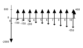
We add inflation by assuming that the general rate of inflation is 6%. In addition we assume that all individual cash flows, including the salvage value, also inflate at 6%. We also add an ordinary tax rate of 25%. We will use straight-line depreciation with 0 tax salvage and a 10-year tax life.

The project is defined by choosing the Add_Project item from the Economics menu. Here we note that both the Inflation and Tax button have been checked.

Selecting Show Cash Flows from the Economics menu builds the cash flow described by the project. The display for this case is shown below. All columns except the last are measured in actual dollars. The second column shows the before-tax cash flow (BTCF) after the inflation factors have been applied. The depreciation column (D) is determined using straight-line depreciation with 0 tax salvage. These values do not reflect inflation because depreciation is not adjusted for inflation. The Tax column is computed by

T = (ordinary tax rate)*(BTCF - D).

The After Tax Cash Flow is: ATCF = BTCF - T.

In the last column, Real Values, the ATCF is converted to real values using the general inflation rate. The values at the top of this display show the NPW and IRR values computed using Excel functions.