Two menu commands are available to compare projects. The first shown, "Compare Projects", compares two projects, and the second "Compare Multiple" compares two or more projects.

Before comparison is possible at least two projects must already reside in the current workbook.

We illustrate this option with an example.

A plant manager is deciding between two machines. Machine A has an initial cost of $9,000. It has no salvage value at the end of its six-year useful life. The annual operating cost of machine A is $5,000. Machine B costs $16,000 new and has a resale value of $4,000 at the end of its nine-year economic life. Its operating costs are $4,000 per year. Do an analysis to determine which machine should be purchased. Assume that operating costs are paid at the end of each year and that the minimum acceptable rate of return is 10%.

The two projects are defined using the Add Project command and appear on the worksheet as below. The projects can be compared by observing their present or uniform annual worths, but the comparison features of the add-in simplifies the process and also provides additional results. The repetition and MARR cells have been filled by the Compare Projects portion of the add-in as will be described later.

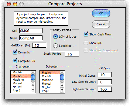
By choosing the Compare Projects option from the menu, we obtain this dialog.

The comparison is given a location on the worksheet and a unique name. The cell indicated is the location of the cursor when the dialog is called. The name must obey the Excel rules for naming ranges. When the LCM, least common multiple, button is selected, the program automatically compares the alternatives for the least common multiples of their lives. A different study period may be selected, but all cash flows falling outside that period are neglected. The collection of projects already defined for the current workbook are listed in the two boxes at the bottom of the dialog. Clicking on one name in each box determines the pair of projects to be compared. The challenger should be the alternative having the greatest initial investment, while the defender should be the one with the least. If the alternatives, both have the same initial investment, choose the one with the earliest investment as the challenger.

Other boxes on the dialog, determine if the display is to be dynamic, whether the IRR is to be computed, whether the cash flow for the incremental investment is to be shown, and characteristics of the cash flow. We illustrate these options below. Clicking OK places the comparison on the worksheet as shown below.

The cells colored yellow in the display hold formulas and should not be changed. The IRR cell is colored green to indicate that this number is computed by an algorithm. The MARR for the comparison is in cell K4 and can be changed to observe the affect on the NPW and NAW of the alternatives. The study period in cell K5 is computed by the user-defined function E_LCM. When a dynamic display is chosen, the MARR and study period in this display is linked by formula to the corresponding values in the projects. At the top of this page, we have noted that the Replication entry for each alternative is determined by a formula that leads to this 18 year study period.Changes in the project data are immediately reflected in this dynamic comparison.

The analysis of the incremental investment of the challenger over the defender is shown near the bottom of the display. We see for the example that the extra investment of B over A returns almost 19%. The increment is certainly justified on this basis as is also indicated by the postitive values of the NPW and NAW.

Since the Show Cash Flow option was chosen, the cash flow for the increment is also placed on the worksheet. The rate shown in cell K22 is computed with the Excel IRR function. The only part of this display that is dynamic is the NPW cell (K20) that changes when the MARR is varied.

If the dynamic box is not selected in the dialog, the display is the same except that it is not linked to the projects being compared. The green cells hold numbers that reflect the data for the two projects, but the numbers do not change as the cash flows for the projects change.

Only one dynamic comparison can be associated with any given project, but any number of non-dynamic comparisons are valid.