 |
The Economics add-in provides convenient
features for modeling cash flow components as random variables.
To use these features have the Random Variables add-in
loaded as well as the Economics add-in. |
Creating a Model |
 |
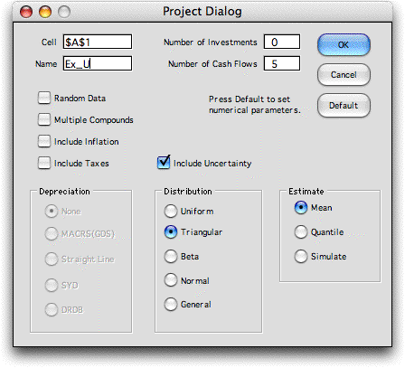
To create a model with uncertainty, choose
the Add Project item from the Economics menu
and click the Uncertainty checkbox on the Project
Dialog as shown below. Select a distribution for the cash
flow components. Clicking a named distribution assigns all
components with the same distribution type. The General button
allows the components to have different distribution types.
The example does not include taxes or inflation, but these
features can also be included when the parameters are uncertain.
A model that includes uncertainty is shown
below. All the cash flow values are assigned triangular distributions.
The example is shown in two parts, but the form on the worksheet
stretches across the worksheet with the cash flow part to the
right of the distribution part. |
|
 |
A model that includes uncertainty
is shown below. All the cash flow values are assigned triangular
distributions. The example is shown in two parts, but the form
on the worksheet stretches across the worksheet with the cash
flow part to the right of the distribution part. |
|
Distribution Description
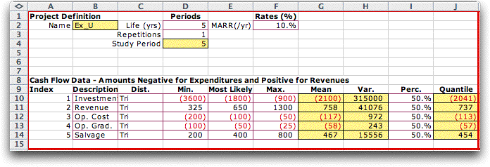
The distribution types are in column C, and
the distribution parameters are in columns D through F.
The Random Variables add-in computes the Mean, Variance and Quantile values
in columns G, H and I, respectively. The Quantiles values
depend on the percentages in column I.
|
Cash Flow Description

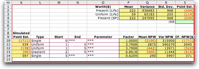
The cash flow information is to the right
of the distribution information. First we explain the
content of rows 10 through 15. Column K holds point estimates
of the component values. Three different point estimates
are available, the Mean Point Estimate, the Quantile
Point Estimate and the Simulated Point Estimate.
The example uses the mean values that are computed in
column G. Characteristics of the cash flow are described
in columns L through O. The equivalency factors are computed
by the Economics add-in in column P. The factors
are used to compute the mean and variance values in
columns Q and R. Column S holds the NPW values
computed using the point estimates.
The results of the analysis are shown in
rows 2 through 6. Row 2 holds the statistical parameters
of the NPW. Cell P2 is the sum of the Mean
NPW values for the components. Cell Q2 is the sum
of Variance NPW values for the components, and
cell R2 is the square root of the variance. Cell S2 is
the NPW computed with the point estimates. Cells
P2 and S2 are the same because the means of the component
distributions are used for as the point estimate in this
case. For quantile point estimates and simulated point
estimates, cells P2 and S2 are usually different.
Row 3 holds the statistical parameters of
the NAW computed from the NPW using the
(A/P, i, N) factor. Row 4 holds the NPW for
the study period. Since the life is the same as the study
period, rows 2 and 4 are identical. The IRR value shown
in cell S5 is the internal rate of return of the
point estimate cash flow. |
Measures of Risk |
 |
If we assume that the NPW is
a normally distributed random variable, we can use the normal
distribution to make probability statements regarding the NPW or NAW.
The figure below shows a form creating by the Random Variables
add-in that describes the distribution of the NPW.
Note we have set the mean and standard deviation of the random
variable, Ex_NPW, equal to the mean and standard deviation
computed for the NPW.
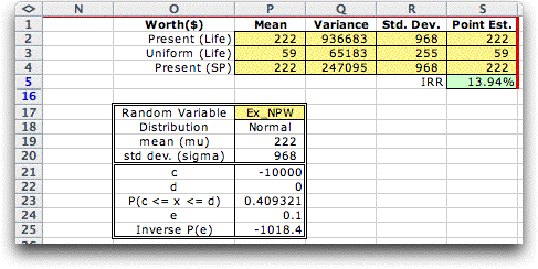
Cell P23 holds a function that computes the probability
that the value falls in the range specified by cells P21 and
P22. The case above shows the probability that the NPW is
less than 0. Cell P25 holds a function that computes the kth
percentile of the random variable. The value of k is
in cell P24. For the case shown, there is a 10% chance that
the NPW will fall below -1,018.4. These are both measures
of risk that may be useful to decision makers when uncertainty
is explicitly modeled. |
Simulation |
| |
When the cash flow component values
are not normally distributed or when other features of the
model are uncertain, simple combinations of means and variances
are not sufficient to obtain valid statistical results. For
these situations, we use Monte-Carlo simulation. The first
step toward simulation is to change the point estimates to
simulated values. This is done by selecting Change Project from
the Economics menu and selecting Simulate from
the point estimate options. Column K in the worksheet below
holds simulated values of the cash flow components. Cell S2
contains the NPW for the simulated values for a single
replication.
|
| |
Choose Simulate_RV from
the Random Variables menu to obtain the dialog below.
Enter S2 as the cell to simulate because it holds the simulated NPW.
The dialog specifies that 1000 observations are to be simulated
and the check boxes indicate the statistics to be gathered.
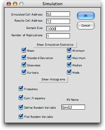
Part of the results of a simulation run are shown
below along with the results computed by the Economics
add-in. The mean and standard deviation obtained by the
simulation are close to those obtained by the previous section
where normality was assumed.

The frequency chart created by the simulation
defines a random variable called SimS2. The name comes
from the address of the simulated cell. Functions available
from the Random Variables add-in compute probabilities
and percentile levels based on the simulated distribution.

Probabilities and percentiles obtained through
simulation do not require the assumption of normality. |
Other Distribution Types |
| |
The figure below shows the statistical
portion of the model when the Beta distribution is chosen
as the default type. Four columns are provided for the parameters
of the Beta distribution. |
|
| |
The form for the general distribution
type provides four columns for parameters, but does not identify
the parameters. Different distributions may be entered for the
components as shown below. The various distributions have different
numbers of parameters ranging from the Fixed distribution
with a single parameter to the Beta distribution with
four parameters. Unused parameters are neglected by the add-in,
but they must be numeric. The example uses 0 for the unused parameters. |
|
Simulating Other Factors |
| |
With the uncertainty features
of the Economics add-in it is easy to model uncertainties
in the individual cash flows. Each cash flow component has a
line on the model display and each line can be assigned a unique
probability distribution. Note that we assume for analysis that
the individual cash flow component values are independent. Also
each multiperiod cash flow such as the uniform series or a gradient
series has the same value of the random variable in each period
of its range.
The are many other factors of the analysis that could be uncertain.
These can be modeled with the help of the Random Variables add-in. The figure below shows an example with various assumed
distributions for the cash flow components. We also assume
that the project life is a random variable with a triangular
distribution. The lower bound is 10 years, the mode is 20 years
and the upper bound is 30 years. The form in the range B22:C26
describes the distribution. |
|
| |
In the cell representing life
we place the function "=RV_SIMV(Life)". This function is provided
by the Random Variables add-in. Each time the worksheet
is computed the life is simulated from the specified distribution.
The cash flow portion of the display is shown below. The
point estimate is simulated in column L. The cash flow parameters
that depend on the life are equations that point to the simulated
value in D2. Every time the worksheet computes, the cash flow
values and the life are simulated and the resultant values
of the present and annual worth are computed. |
|
| |
The figure below shows the histogram
from 1000 simulated observations.

Any number of independent uncertain factors can
be modeled in this way. |
| |
|


