|
|
 |
Investment
Economics |
 |
-Inflation
|
 |
The add-in can also be used to analyze economic investments
with price inflation. The inflation analysis is available
with or without taxes. We repeat the example used earlier,
but add the effects of inflation. We first neglect tax considerations.
In this section, we show how to describe and compare projects
when price inflation is present. We assume that the user has
some idea of the notation and concepts associated with inflation.
A businessman is considering the purchase of an asset that
has an initial cost of $2000. The asset promises an annual return
of $600. It's operating cost is $100 the first year, $150 the
second, and increases by $50 in each subsequent year. The salvage
value for the asset in 10 years is $400.
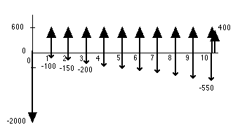
We add inflation by assuming that the general
rate of inflation is 6%. In addition we assume that all individual
cash flows, including the salvage value, also inflate at 6%.
Again we will accept the project if it satisfies the minimum
accepted rate of return of 10%. When inflation is present, we
must specify that this is the MARR in "real" terms.
The project is defined by choosing the Add_Project
item from the Economics menu. Here we note that the Inflation
button has been checked for the example, but the Tax
button is unchecked. |
| |
|
Project Definition |
| |
On clicking OK, the project definition
appears on the worksheet. Several new data items and result
items appear on the form. In column H near the top of the form
there are two entries for the MARR. The Real MARR is
entered as data in H9 and the Actual (or Market)
MARR is computed in cell H10. An estimate for the
general inflation rate is in cell H11.
In the lower half of the
display a new column, column J for the example, is added for
both investment data and cash flow data segments. The new column
holds an incremental inflation rate for each component
of the cash flow. This entry shows the difference between the
general inflation rate and the escalation rate for each component.
The incremental rate is positive is the escalation rate is
greater than the general inflation rate and negative if the
escalation rate is less than the general inflation rate. For
this example we have entered 0% indicating that all components
escalate at the same rate as general inflation. |
| |

Click the image to expand |
| |
The numbers placed in the Amounts column
are the values of the cash flows estimated at "today's" prices.
When an escalation rate is greater than 0, the actual dollar
expenditures or revenues grow as a function of the time they
occur. When the cash flow is measured in terms of the dollars
at the time of the cash flow, the measure is called actual dollars.
A real dollar value is the actual
dollar value reduced to remove the effect
of general inflation. Formulas relating the three measures
are below.
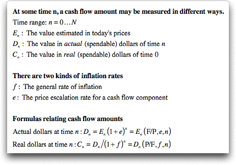
The rightmost column shows the equivalent value,
or the present worth, of the project at time 0. At time 0, real
and actual dollars are the same. |
Rates
of Return |
| |
At the top of the display
we place new quantities that relate specifically to inflation
analysis.
Real MARR:
This is the minimum acceptable rate of return when returns
are measured in real dollars. This quantity may be changed
and the Worth column will automatically adjust.
Actual MARR:
This is the minimum acceptable rate of return when returns
are measured in actual dollars. This quantity is computed
using the formula below. The quantity will change automatically
when either the real MARR or the general inflation rate changes.
General Inflation:
This is the average inflation rate for comparing real and
actual dollars.
An investor desires to earn an interest rate the provides
a reward for giving up money, but the investor also must earn
an amount that compensates for the loss in value due to inflation.
The real MARR is the minimum acceptable rate to be
earned if there were no inflation, while the actual (or
market) MARR includes an allowance for inflation. The relations between
the two quantities are given in the equations below.

|
Worth
Measures |
| |
At the right of the display we show several
measures of the worth of the project.
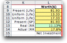
Present Worth: This is the value of the project at
time 0 when all cash flows are replaced by their equivalent
values at time 0. The value is the same whether measured in
actual or real dollars.
Real Uniform (Life): This is the uniform annual equivalent
(NAW) of the present worth when it is spread over the life
of the project using the real MARR.
Actual Uniform (Life): This is the uniform annual equivalent
(NAW) of the present worth when it is spread over the life
of the project using the actual MARR.

For most situations the real NAW is the best
measure of annual costs.
Present Worth(SP): This is the present
worth considering only the cash flows within some study period
that may be more or less than the life. The study period may
be different from the life when several replicas of the project
are repeated as when comparing two projects of different lives.
In some situations it may be useful to set the study period
as less than the life of the project.
Real IRR: This is the internal rate of
return when cash flows are measured in real dollars. It should
be compared to the real MARR. The cell is shown in green to
indicate that it is a computed quantity. Choose Compute
Rates from the Economic menu to compute the rate.
This is not a dynamic quantity and it must be re-computed whenever
the data is changed.
Actual IRR: This is the internal rate
of return when the cash flows are measured in actual dollars.
It is computed directly from the real IRR using the general
inflation rate and a formula similar to the formula shown above
relating the real and actual MARR values.
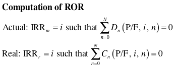
For the example, all the measures show that this
project makes more than the required MARR. All present and
annual worth's are positive, and the IRR values are both greater
than the minimum acceptable rates or return. |
Cash Flows |
| |
Selecting Show Cash Flows from the Economics menu
builds the cash flow described by the project. When inflation
is included in the model, columns are provided for both the actual
and real cash flows. The NPW and IRR values are computed directly
from the cash flows using built-in Excel functions. They should
agree with the values computed by the add-in on the project display.
The example shows the effects of inflation. For the example,
all cash flows had the same inflation rate as general inflation.
In this case the real cash flow is the same as the estimated
cash flow. The payback period is computed using the Cumulative
Real Values, shown in the column on the right. |
|
| |
With inflation, there is a difference between
real and actual cash flows. The graphical display shows actual
revenues as black lines and real revenues as green lines. Actual
disbursements are shown as red lines and real disbursements as
maroon lines. The investment at time 0 is the same in both real
and actual dollars. The real color is foremost, so only the maroon
line shows. |
| |
|
When Inflation
Rates are Different |
| |
To illustrate the effects of
different inflation rates, we modify the example as below with
a variety of assumptions about the price escalation rates for
the components. Click the figure to see a larger version of
the form created by the add-in.

Click the image to expand |
We are assuming a general inflation rate
of 6%. Escalation rates for the components of the investment
and cash flow items are entered as differences from the general
inflation rate, or as incremental
inflation rates. Here we see that
the initial cost line has an incremental inflation rate of
4%. This means that the
initial cost is escalating at a rate of 6% + 4% = 10%. Because
the initial cost is expended at time 0, inflation has no
effect on this value. The salvage value will, however, escalate
at the 10% rate. Instead of being $400, as estimated
in today's prices, the salvage will increase in actual dollars
at a rate of 10% per year. The factor
value for the row reflects both the 20% salvage estimate
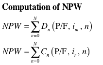
and the 10% price escalation. The equations
below indicate how the NPW representing the initial cost
is computed.
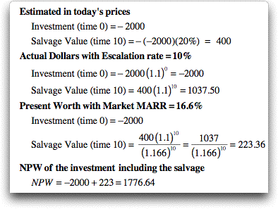
For our example, we assume that the returns
for the project escalate at a rate of 7%, that is, 1% greater
than general inflation. Since this is a uniform series when
estimated in today's prices, the return measured in actual
dollars will be increase with time. The return in one year
when measured in actual dollars is equal to (1.07) times the
value in the previous year. The uniform series representing
operating cost is growing at a 4% rate, that is 2% less than
general inflation. We assume that the gradient component is
constant in actual dollars, so the escalation rate is 0 and
the incremental inflation rate is -6%. The factors computed
by the add-in and shown in the factor column of the
form adjust the cash flows for the inflationary effects. The
NPW values are computed in the right-most column.
The results of the analysis are
computed at the upper right of the form. With the assumed
parameters, the project has the NPW of $741. The positive value
indicating that the project returns more than the MARR. There
are two kinds of Uniform Worth. The first, in cell L31, is
the NAW computed using the real MARR. This value is the uniform
equivalent expressed in real dollars. The second, in cell L32,
is the NAW computed using the market MARR. This value is the
uniform equivalent expressed in actual dollars. Cell L33 holds
the NPW for the study period. For the example the study period
is the same as the life. Cell L34 holds the IRR of the project
using real cash flows, while L35 is the IRR computed with the
actual cash flows. Both exceed their respective MARR values.
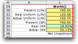
Although the table above shows six measures for
the worth of the project, they all give the same decision.
They all indicate that the project is acceptable. For simple
investments, the measures always give the same results. For
non-simple investments where there are multiple values for
the IRR, use of the RIC rather that the IRR resolves that ambiguity.
We provide so many measures because they are useful in different
contexts. Most decision makers probably prefer the Actual IRR
as a measure because they are familiar with rates of return
and most rates are expressed as market rates.
The cash flow for this example is shown below. |
| |
|
Comparing Projects |
| |
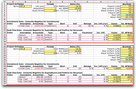
To compare two projects, they both must include
inflation parameters. For an example, two projects are shown
below. We compare them by choosing Compare Projects from
the Economics menu. To compare more projects than two,
choose Compare Multiple from the menu. The examples from
this section are from and earlier version of the add-in. |
Click the image to expand
|
|
| |
The comparison controls the Real MARR, in cell
L4 for this example. We have used Infl_B as the challenger and
Infl_A as the defender, because Infl_B has the greater initial
investment. The extra investment yields a real return of 15.4%
and it is certainly justified when the real MARR is 10%. The
cash flow of the comparison shows the difference between the
two alternatives. |
| |
|
| |
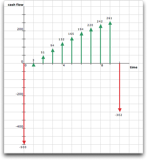
The graph shows the incremental cash flow of
Infl_B over Infl_A. The graph was constructed by the add-in.
|
| |
|
|


