Computation Section
Investment Economics
 -Simulation


The other pages of this section assume all features of the economic project are certain. This is not a very reasonable assumption, because all of the parameters of the model estimate future events. These are by their nature often very uncertain.

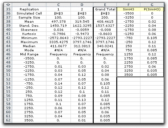
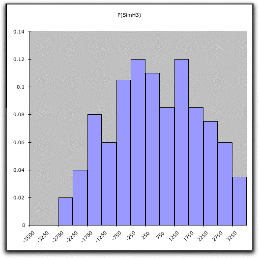
One way to deal with uncertainty is to propose probability models for the parameters of the system and find statistical estimates for the profitability 
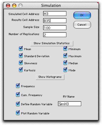
of the project using Monte Carlo simulation. By combining the capabilities of the Economics and Random Variables add-ins, we can simulate many of the features of the model. Both add-ins must be installed to duplicate the operations described on this page. The demonstration file for this page is called Ecosim.xls. You may download this file and follow along the steps.

Since the demonstration file was created on the author's computer, it is necessary to use the Refresh Functions commands on both the Economics and Random Variables menus.

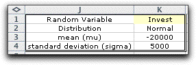
We start by adding a project using the Add Project command on the Economics menu. The example below uses the default parameters.

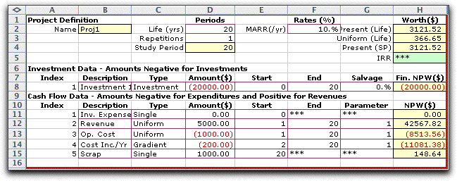
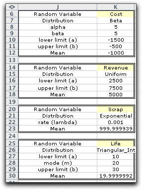
This model has all parameters fixed, but we will replace some of them with random variables.


Creating the random variables


We first create a random variable for the investment. We do this by choosing the Add RV command from the Random Variables menu. The dialog presented below has a field for the cell at which the random variable parameters will be placed (Cell J1) for the example. The dollar signs are not necessary. The Name is important because it will be referenced by the simulation model. Any of the 19 distributions may be chosen. The requisite parameters are entered in the data fields. These parameters can be changed directly on the worksheet, but the name is fixed once the probability model is placed on the sheet.

The random variable definition is placed on the worksheet starting in J1. Random variables may be placed in any convenient location. The parameters for the random variables can be changed on this form, but the name should not be changed. Note that we have specified the mean of the random variable as -20000. We use a negative sign because the investment is a cash flow out.

We decide to create random variables for several other parameters as shown below.

We have chosen a discrete distribution for the life since the economic model assumes discrete compounding. The other parameters have a variety of continuous distributions.


Linking to the Economic Form


We link the parameters on the project form using the RV_SimV function. This is a user defined function from the Random Variables add-in that provides a simulated value from the distribution named in its single argument. The simulation uses the Monte Carlo method. We replace the parameter values with the function calls as in the figure below.

The V that appears as the last letter of RV_SIMV stands for volatile. Every time the worksheet recalculates a new set of simulated values is generated. You can test this by pressing the Ctrl and = keys simultaneously. This does a worksheet calculation. All the random variables will change.


Simulate

 
Note that the uniform worth of the project is in cell H3. This is a reasonable result to simulate since one of the random variables is the life of the project. We simulate by selecting the Simulate command from the Random Variables menu.

The simulate dialog accepts the desired features of the simulation. The simulated cell is H3. The results cell is important because we want to put the results at some location on the worksheet that will not overwrite other information. The default value is just to the right of the simulated cell. If this option were accepted all the random variable definitions would be overwritten. We have selected B35. The checkboxes indicate the results that are to be displayed.


Clicking the OK button initiates the simulation. After the first replication of 100 observations a dialog box is presented with some of statistics for the current run. These are used to set the parameters of the histogram that is to be compiled at the end of the run. We have changed the default values of the lower and upper limits to obtain a more useful histogram.


Simulation Results


In a few seconds the simulation is complete and the results are shown on the worksheet. The descriptive statistics are on rows 38 through 45. The histogram cell frequencies are on rows 47 through 62. The cumulative frequencies, not shown, start at row 63.


The last two columns define a random variable called SimH3. This random variable can be used for additional studies. It is the source of the chart shown below. The chart appears to the right of the distribution results.

Although a mean value analysis suggests that the project will meet the MARR requirement of 10%. There is a good chance that the annual worth will be negative. This means that the project may well yield a rate of return less than the minimum.

  The ability to simulate the components of a cash flow provides a useful approach to modeling uncertainty. Any results that are dynamically linked to cells that can effect their values can be simulated with this Monte Carlo method.
 
  
Return to Top

tree roots

Operations Management / Industrial Engineering
Internet
by Paul A. Jensen
Copyright 2004 - All rights reserved

Next Page