Operation - Operations Management / Industrial Engineering

Operation

Inventory

General

Deterministic

No Shortages
Infinite
Finite

Shortages Backordered
Infinite
Finite

Lost Sales
Infinite
Finite

Summary

	Inventory Theory
	- Deterministic/No Shortages/Finite Replenishment

In this section we consider a system similar to the system on the previous page except here product is added to the inventory at a finite rate, rather than arrive instantaneously as in the previous model.

The model with finite replenishments is illustrated below. Rather than arrive instantaneously, the lot is assumed to arrive continuously at a rate P. This situation arises when a production process feeds the inventory and the process operates at the rate P. Of course P must be greater than the demand rate D.

Time when production stops:

A more detailed picture of a cycle illustrates some important points.The maximum inventory level never reaches q because material is withdrawn at the same time it is being replenished. Replenishment takes place at the beginning of the cycle when the inventory grows at the rate P-D. At time t’ production stops. For the remainder of the cycle, inventory is withdrawn at a rate D, the demand rate,.until it reaches 0 at the end of the cycle.

Formulas for Instance Results

Click buttons to see the notation

Here we derive the formulas for the results for an instance. An instance is defined by a collection of inventory parameters and a value for the lot size q. Click the buttons on the left for a description of the notation for parameters and results.

These formulas are implemented in the Inventory add-in.

To construct a mathematical model describing the economic costs or profits associated with the inventory system, we show the cash flows below. This figure is a mixed representation of discrete as well as continuous cash flows. The arrows represent amounts paid or received at points in time. The areas represent continuous cash flows given by rates. Amounts appearing above the 0 axis are revenues, while amounts below are expenditures or costs.

The table below shows the various revenue and cost components and their respective cost rates.

Item	Amount during a cycle	Cost or revenue rate
Ordering Cost In each cycle an order is placed for the quantity q	A
Product Cost	Cq=CPt'
Holding Cost for Product in Inventory	Average Inventory * H
Revenue from product Sales	Rq	RD

For this model there is a single decision variable that is the lot size or the replenishment, q. All other quantities are a function of q. We assume that all parameters are nonnegative and that P > D. The inventory cost is a convex function of q.

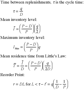
Additional quantities associated with the inventory policy are derived below.

The reorder point calculation assumes that a replenishment order will take place when the system is not producing and the inventory level is decreasing at the rate of demand. If the lead time is longer than the upper limit in the equation, a more complex equation is necessary to compute the reorder point. The add-in uses the more complex equation that computes the reorder point for an arbitrary lead time.

The measures are computed below for the example using a lot size of 400 units. This is called an instance of the inventory model. The figure shows a single cycle of the inventory pattern.

Optimum Policy

For determination of the optimum lot size q*, the unit revenue and unit cost can be neglected and we write the expression for the cost rate for operating the inventory.

When q* is between the minimum and maximum lot sizes, the inventory measures with the optimum lot size are found by substituting q* into the instance formula.

The optimal lot size increases with increasing setup cost and flow rate and decreases with increasing holding cost. As P approaches D the optimal lot size approaches infinity and the inventory cost goes to zero.

The table below shows the instance results as well as the results for the optimum lot size (q*= 1155). This example has the same parameters as the infinite case except the finite replenishment rate. Observe that the optimum lot size has increased from 815 to 1155.